Contents

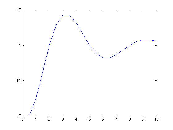
Euler method

clear all

xi = 0.5;
A = [0 1; -1 -2.0*xi];
B = [0; 1];

N = 21;
u = linspace(0,10,N);

x = [0;0];
du = u(2)-u(1);
y = zeros(size(u));

for n=1:N
    y(n) = x(1);
    dx = (A*x + B)*du;
    x = x + dx;
end

plot(u,y);

Exact solution (underdamped xi <1)

xi = 0.5;
vf = 1;
wn  = sqrt(1-xi^2);
A = [ 1 0; -xi wn ];
b = [-vf; 0];
K = A\b;

ye = vf + (K(1)*cos(wn*u) + K(2)*sin(wn*u)).*exp(-xi*u);

plot(u,ye);

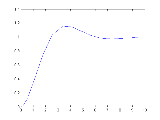
Runge-Kutta

    x = [0;0];
    yr = zeros(size(u));
    err = zeros(size(u));
    h = u(2) - u(1);
    for n=1:N
       t = u(n);
       yr(n) = x(1);
       k1 = deriv(t, x) * h;
       k2 = h * deriv(t + h/3.0, x + k1/3.0);
       k3 = h * deriv(t + h/3.0, x + k1/6.0 + k2/6.0);
       k4 = h * deriv(t + h/2.0, x + k1/8.0 + (3.0/8.0)*k3);
       k5 = h * deriv(t + h, x + k1/2.0 - 1.5 * k3 + 2.0 * k4);
       errx = (2.0*k1 - 9.0*k3 + 8.0*k4 - k5)/30.0;
       err(n) = errx(1);
       dx = (k1 + 4.0*k4 + k5)/6.0;

       x = x + dx;
    end

    plot(u,yr);

MATLAB ODE45

ysolve = ode45(@deriv,[0 10],[0;0]);
tm = ysolve.x;
ym = ysolve.y(1,:);

plot(tm,ym);

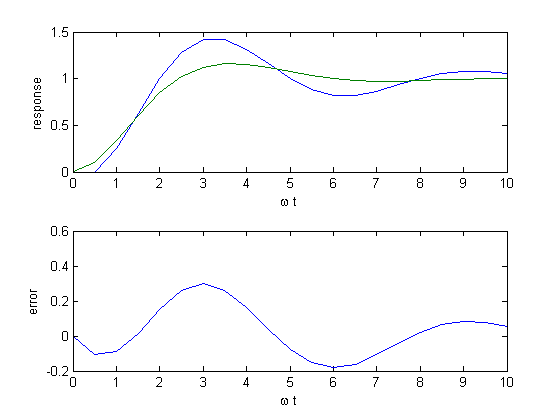
Compare exact with Euler

subplot(2,1,1);
plot(u, y, u, ye);
xlabel('\omega t');
ylabel('response');
subplot(2,1,2);
plot(u,y-ye);
xlabel('\omega t');
ylabel('error');

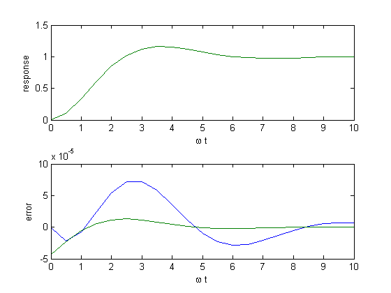
Compare exact with Runge-Kutta

subplot(2,1,1);
plot(u, yr, u, ye);
xlabel('\omega t');
ylabel('response');
subplot(2,1,2);
plot(u,yr-ye,u,err);
xlabel('\omega t');
ylabel('error');

Published with MATLAB® 7.4