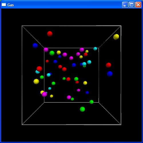
A model of an ideal gas with hard-sphere collisions The program uses Numeric Python arrays for high speed computations
This is an example from the VPython distribution
gas.py001: from visual import * 002: from time import clock 003: from visual.graph import * 004: from random import random 005: 006: # A model of an ideal gas with hard-sphere collisions 007: # Program uses Numeric Python arrays for high speed computations 008: 009: win=500 010: 011: Natoms = 50 # change this to have more or fewer atoms 012: 013: # Typical values 014: L = 1. # container is a cube L on a side 015: gray = (0.7,0.7,0.7) # color of edges of container 016: Raxes = 0.005 # radius of lines drawn on edges of cube 017: Matom = 4E-3/6E23 # helium mass 018: Ratom = 0.03 # wildly exaggerated size of helium atom 019: k = 1.4E-23 # Boltzmann constant 020: T = 300. # around room temperature 021: dt = 1E-5 022: 023: scene = display(title="Gas", width=win, height=win, x=0, y=0, 024: range=L, center=(L/2.,L/2.,L/2.)) 025: 026: deltav = 100. # binning for v histogram 027: vdist = gdisplay(x=0, y=win, ymax = Natoms*deltav/1000., 028: width=win, height=win/2, xtitle='v', ytitle='dN') 029: theory = gcurve(color=color.cyan) 030: observation = ghistogram(bins=arange(0.,3000.,deltav), 031: accumulate=1, average=1, color=color.red) 032: 033: dv = 10. 034: for v in arange(0.,3001.+dv,dv): # theoretical prediction 035: theory.plot(pos=(v, 036: (deltav/dv)*Natoms*4.*pi*((Matom/(2.*pi*k*T))**1.5) 037: *exp((-0.5*Matom*v**2)/(k*T))*v**2*dv)) 038: 039: xaxis = curve(pos=[(0,0,0), (L,0,0)], color=gray, radius=Raxes) 040: yaxis = curve(pos=[(0,0,0), (0,L,0)], color=gray, radius=Raxes) 041: zaxis = curve(pos=[(0,0,0), (0,0,L)], color=gray, radius=Raxes) 042: xaxis2 = curve(pos=[(L,L,L), (0,L,L), (0,0,L), (L,0,L)], color=gray, radius=Raxes) 043: yaxis2 = curve(pos=[(L,L,L), (L,0,L), (L,0,0), (L,L,0)], color=gray, radius=Raxes) 044: zaxis2 = curve(pos=[(L,L,L), (L,L,0), (0,L,0), (0,L,L)], color=gray, radius=Raxes) 045: 046: Atoms = [] 047: colors = [color.red, color.green, color.blue, 048: color.yellow, color.cyan, color.magenta] 049: poslist = [] 050: plist = [] 051: mlist = [] 052: rlist = [] 053: 054: for i in range(Natoms): 055: Lmin = 1.1*Ratom 056: Lmax = L-Lmin 057: x = Lmin+(Lmax-Lmin)*random() 058: y = Lmin+(Lmax-Lmin)*random() 059: z = Lmin+(Lmax-Lmin)*random() 060: r = Ratom 061: Atoms = Atoms+[sphere(pos=(x,y,z), radius=r, color=colors[i % 6])] 062: mass = Matom*r**3/Ratom**3 063: pavg = sqrt(2.*mass*1.5*k*T) # average kinetic energy p**2/(2mass) = (3/2)kT 064: theta = pi*random() 065: phi = 2*pi*random() 066: px = pavg*sin(theta)*cos(phi) 067: py = pavg*sin(theta)*sin(phi) 068: pz = pavg*cos(theta) 069: poslist.append((x,y,z)) 070: plist.append((px,py,pz)) 071: mlist.append(mass) 072: rlist.append(r) 073: 074: pos = array(poslist) 075: p = array(plist) 076: m = array(mlist) 077: m.shape = (Natoms,1) # Numeric Python: (1 by Natoms) vs. (Natoms by 1) 078: radius = array(rlist) 079: 080: t = 0.0 081: Nsteps = 0 082: pos = pos+(p/m)*(dt/2.) # initial half-step 083: time = clock() 084: 085: while 1: 086: observation.plot(data=mag(p/m)) 087: 088: # Update all positions 089: pos = pos+(p/m)*dt 090: 091: r = pos-pos[:,NewAxis] # all pairs of atom-to-atom vectors 092: rmag = sqrt(add.reduce(r*r,-1)) # atom-to-atom scalar distances 093: hit = less_equal(rmag,radius+radius[:,NewAxis])-identity(Natoms) 094: hitlist = sort(nonzero(hit.flat)).tolist() # i,j encoded as i*Natoms+j 095: 096: # If any collisions took place: 097: for ij in hitlist: 098: i, j = divmod(ij,Natoms) # decode atom pair 099: hitlist.remove(j*Natoms+i) # remove symmetric j,i pair from list 100: ptot = p[i]+p[j] 101: mi = m[i,0] 102: mj = m[j,0] 103: vi = p[i]/mi 104: vj = p[j]/mj 105: ri = Atoms[i].radius 106: rj = Atoms[j].radius 107: a = mag(vj-vi)**2 108: if a == 0: continue # exactly same velocities 109: b = 2*dot(pos[i]-pos[j],vj-vi) 110: c = mag(pos[i]-pos[j])**2-(ri+rj)**2 111: d = b**2-4.*a*c 112: if d < 0: continue # something wrong; ignore this rare case 113: deltat = (-b+sqrt(d))/(2.*a) # t-deltat is when they made contact 114: pos[i] = pos[i]-(p[i]/mi)*deltat # back up to contact configuration 115: pos[j] = pos[j]-(p[j]/mj)*deltat 116: mtot = mi+mj 117: pcmi = p[i]-ptot*mi/mtot # transform momenta to cm frame 118: pcmj = p[j]-ptot*mj/mtot 119: rrel = norm(pos[j]-pos[i]) 120: pcmi = pcmi-2*dot(pcmi,rrel)*rrel # bounce in cm frame 121: pcmj = pcmj-2*dot(pcmj,rrel)*rrel 122: p[i] = pcmi+ptot*mi/mtot # transform momenta back to lab frame 123: p[j] = pcmj+ptot*mj/mtot 124: pos[i] = pos[i]+(p[i]/mi)*deltat # move forward deltat in time 125: pos[j] = pos[j]+(p[j]/mj)*deltat 126: 127: # Bounce off walls 128: outside = less_equal(pos,Ratom) # walls closest to origin 129: p1 = p*outside 130: p = p-p1+abs(p1) # force p component inward 131: outside = greater_equal(pos,L-Ratom) # walls farther from origin 132: p1 = p*outside 133: p = p-p1-abs(p1) # force p component inward 134: 135: # Update positions of display objects 136: for i in range(Natoms): 137: Atoms[i].pos = pos[i] 138: 139: Nsteps = Nsteps+1 140: t = t+dt 141: 142: if Nsteps == 50: 143: print '%3.1f seconds for %d steps with %d Atoms' % (clock()-time, Nsteps, Natoms) 144: ## rate(30)