ECE 563 Assignment 7
Images and matlab functions for this assignment may be downloaded from
impro7.zip.
- Download the multispectral images from wva1_TM.zip.
Find the three strongest principal components. Use the strongest as I, and the next
two as X and Y. You may need to scale I to the range 0..1 and (X, Y) to -1 .. 1.
Convert XYI to RGB and show the result. Take the RGB image, convert to HSV, and rotate
the H component so that green seems to denote vegetation when the rotated HSV is converted
back to RGB. Show your final RGB image.
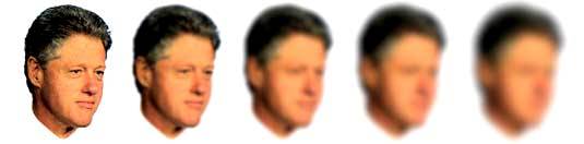
- Generate progressively blurred sets of images, similar to that shown below, using different
averaging filters (e.g. flat, gaussian, binomial). To make the problem current, use an image of
your favorite (or least-faviorite) Presidential candidiate. The handout has a selection of possible
starting images.
- Let a gaussian image with standard deviation s1 be
filtered with a gaussian averaging filter with standard deviation s2.
Find the standard deviation of the resulting image. Do analyically and verify numerically.
- Calculate the mean and standard deviation of graycard_75dpi (from impro3.zip) as
a function of the number of times a certain averaging filter is applied (flat, gaussian, binomial).
- Find the best-fitting gaussian for binomial filters of order n=2..10. Show plots
of the (continuous) gaussian and the (discrete) binomial filter weights for each order.
- Generate a set of grayscale images using increasing amounts of salt-and-pepper noise (using
the matlab function imnoise). Show the improvement (if any) after filtering with smoothing
filters and median filters (see medfilt2). Evaluate the degree of improvment obtained,
by calculating the statistics of the differences between the original image and both the degraded
and improved images.
- Choose an image, convert it to grayscale, and display (a) the
original grayscale image (b) magnitude of gradient image, (c) Laplacian filtered image, and
(d) Morphological gradient image (min/max).
- Prepare Powerpoint and published MATLAB tutorials on the following topics
(see Using Deblurring in IPT Help):
- Group 1: blind deconvolution, deconvblind
- Group 2: Lucy-Richardson, deconvlucy
- Group 3: Regularized filter, deconvreg
- Group 4: Wiener filter wiener2 and deconvwnr.
Provide as many details as you can find (examine the matlab source) about each method, and give
examples of its use.
Maintained by John Loomis,
last updated 10 March 2016