Univariate image statistics apply to single-band images.
The histogram of an image plots the frequency of occurrence (count) of gray levels for each gray level present in the image. For a continuous image, the gray scale is partitioned into equally-spaced bins and each pixel is assigned an appropriate bin index (gray level). Each bin counts the number of pixels in the image having the corresponding bin index.
In matlab, the function imhist can be used to generate and display image histograms.
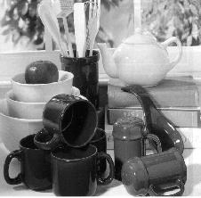
ģ im = imread('kitchen2.tif');
ģ imshow(im);
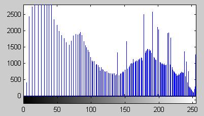
ģ imhist(im);
One interesting observation in this example is that the gray levels are not uniformly populated.
The first few central moments of an image histogram are given by
| mean |  |  |
|---|---|---|
| variance |  |  |
| skewness |  | |
| kurtosis |  |
Skewness measures the asymmetry of a distribution. It is positive if there is a long tail to the right and negative for a tail on the left.
Kurtosis measures the sharpness of the distribution relative to a Gaussian distribution. Negative kurtosis implies that the peak is broader than a Gaussian. Positive kurtosis means that the distribution is sharper than a Gaussian.
Skewness and kurtosis are sensitive to outliers, pixels with gray levels far removed from the majority distribution.
The normal (Gaussian) distribution has the form
There are two common textbook definitions for the variance s2 of a data vector Z:

where m is the mean and N is the number of elements in the sample. The two forms of the equation differ only in N versus N-1 in the divisor. If Z is a random sample of data from a normal distribution, the expression with N-1 is the best unbiased estimate of its variance. The expression involving N is often used in the defintion of the moments of a probability distribution. For most images, N is so large that both expressions are equivalent.
The histogram can be used to simplify the calculation of the statistical moments
where f(k) is the histogram, k is the bin index (gray level), and K is the number of gray levels.
There are a variety of expressions for the range or contrast of an image and image modulation.
The mid-range, Zmax + Zmin, of a bipolar image can be zero. In this case, the definition of mid-range can be extended through the use of absolute value signs, as shown below
The maximum possible range, or maximum number of gray levels, could also be used in the denominator.
function imstats(im)
%
%  Calculate image statistics
%

[counts, x] = imhist(im);
N = sum(counts);

f = find(counts);
n = length(f);
nlevels = length(x);
if (n<nlevels)
   disp(sprintf('Image has %d of %d possible levels\n',n, nlevels));
end

z = im2double(im);
% contrast
zmax = max(max(z));
zmin = min(min(z));
range = zmax-zmin;
modulation = range/max(abs([zmin zmax]));
disp(sprintf('    zmax\t    zmin\t   range\t  contrast'));
disp(sprintf('%8.4g\t%8.4g\t%8.4g\t%10.4g\n',zmax,zmin,range,modulation));


% moments
avg = mean2(z);
z = z - avg;
sig = sqrt(mean2(z.*z));
z = z/sig;
skewness = mean2(z.^3);
kurtosis = mean2(z.^4)-3;

disp(sprintf('    mean\t     std\t  skewness\t  kurtosis'));
disp(sprintf('%8.4g\t%8.4g\t%10.4g\t%10.4g',avg,sig,skewness,kurtosis));
ģ im = imread('kitchen2.tif');
ģ imstats(im)
Image has 145 of 256 possible levels
zmax zmin range contrast
255 1 254 0.996078
mean std skewness kurtosis
130.686 72.9996 -0.137485 -1.33379
ģ [out, rect] = imcrop(im);
ģ imwrite(out,'sample.jpg');
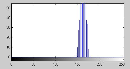
ģ imhist(out);
ģ imstats(out)
Image has 25 of 256 possible levels
zmax zmin range contrast
180 144 36 0.2
mean std skewness kurtosis
162.292 5.0482 0.0767204 0.0996876

Maintained by John Loomis, last updated 2 Jan 2001