Ortho

Produce orthonormal view from oblique projective image

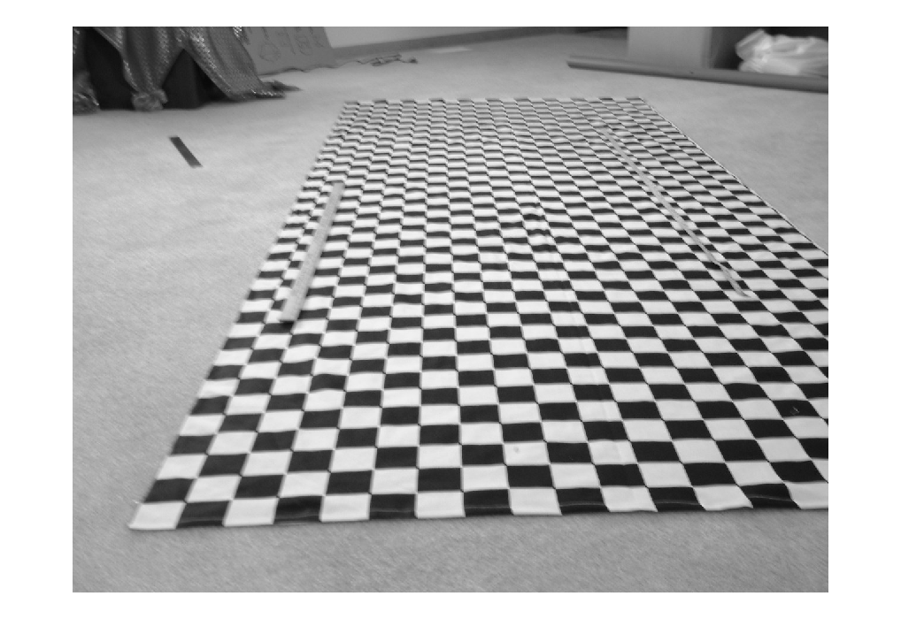
read original image

clear; close all
filename = '2002_1229_125739AA.JPG';
img = im2double(rgb2gray(imread(filename)));
name = 'check2';
msgid = 'Images:initSize:adjustingMag';
warning('off',msgid);
imshow(img);

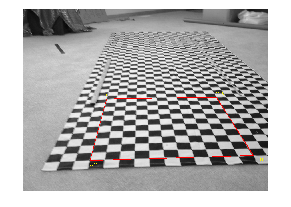
input corners (using impixel) and compute transform

%[c r p] = impixel;
c = [ 349 1207 1012 436 ]';
r = [ 800  773  466 476 ]';
base = [0 11; 11 11; 11 0; 0 0];
tf = cp2tform([c r],base*80,'projective');
disp('tf = ');
disp(tf)
disp('tf.tdata = ');
disp(tf.tdata);

T = tf.tdata.T;
disp('T =');
format short g
disp(T);
format

tf = 
       ndims_in: 2
      ndims_out: 2
    forward_fcn: @fwd_projective
    inverse_fcn: @inv_projective
          tdata: [1x1 struct]

tf.tdata = 
       T: [3x3 double]
    Tinv: [3x3 double]

T =
       1.4961     0.071194  -1.7051e-05
      0.40173       4.1008    0.0015472
      -843.53        -1983      0.27095

overlay control points on image

imshow(img);
hold on;
plot([c;c(1)],[r;r(1)],'r','Linewidth',2);
text(c(1),r(1)+20,'0, 11','Color','y');
text(c(2),r(2)+20,'11, 11','Color','y');
text(c(3),r(3)-20,'11, 0','Color','y');
text(c(4),r(4)-20,'0, 0','Color','y');
hold off;
F = getframe();
g = frame2im(F);
imwrite(g,[name '_overlay.jpg']);

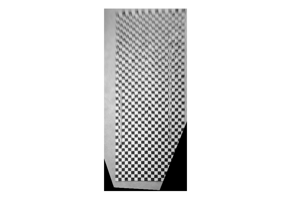
do image transform

[xf1, XData, YData] = imtransform(img,tf);
imshow(xf1)
imwrite(xf1,[name '_registered.jpg']);

Warning: IMTRANSFORM has increased the scale of your
output pixels in X-Y space to keep the dimensions of
the output image from getting too large. This
automatic scale change will be removed in a future
release.
To ensure that output pixel scale matches input
pixel scale specify the 'XYScale' parameter. For
example, call IMTRANSFORM  like this:

     B = IMTRANSFORM(A,T,'XYScale',1) 

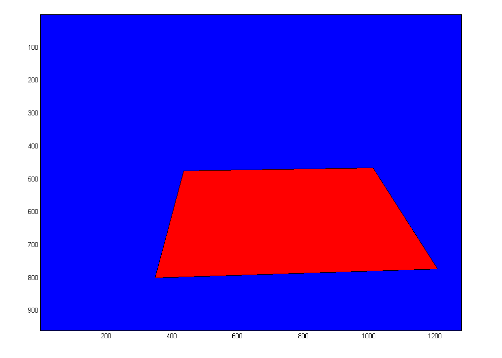
show a simplified form of the original image

bdi = [1 1; 1280 1; 1280 960; 1 960];
fill(bdi(:,1),bdi(:,2),'b');
axis ij;
hold on
fill(c,r,'r');
hold off
axis equal

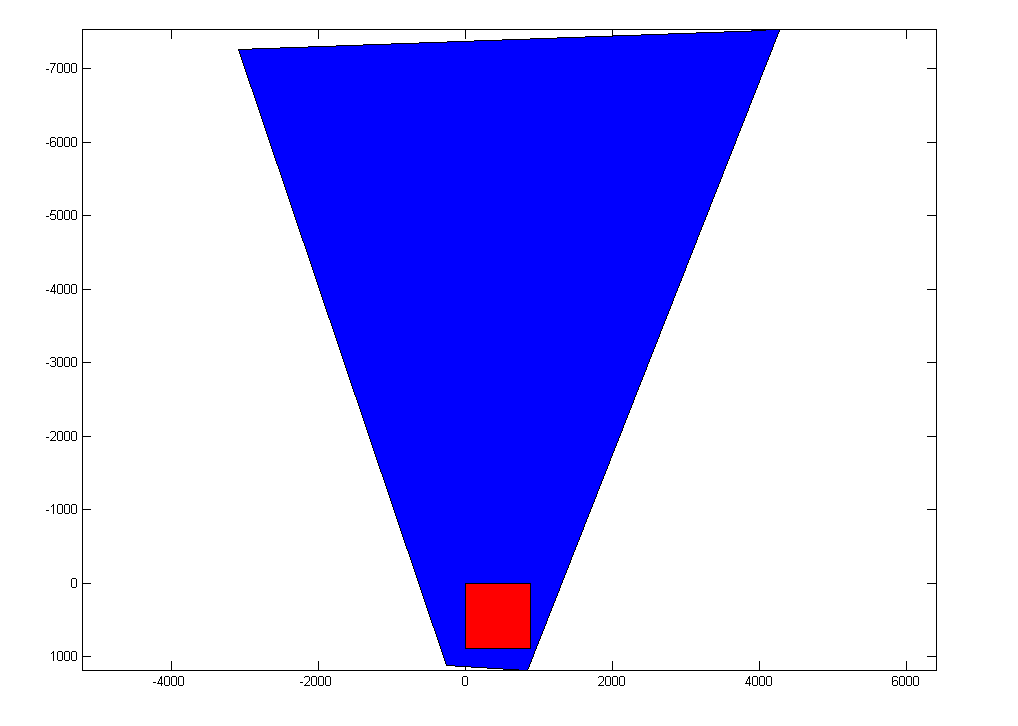
% show the transformed simplified image
rd = tformfwd(tf,[c r]);
bds = tformfwd(tf,bdi);
fill(bds(:,1),bds(:,2),'b')
axis ij
hold on
fill(rd(:,1),rd(:,2),'r')
axis equal
hold off

% show that the control points map to the target points
prd = [c r ones(4,1)]*T;
% B = repmat(A,M,N) creates a large matrix B consisting of an M-by-N
%     tiling of copies of A.
%  This is used to produce two copies of the the third, homogeneous
%  variable. The end result is to convert homogeneous to normal variables.
uv = prd(:,1:2)./repmat(prd(:,3),1,2);
disp('uv/80 = ');
disp(uv/80)

uv/80 = 
   -0.0000   11.0000
   11.0000   11.0000
   11.0000         0
   -0.0000   -0.0000

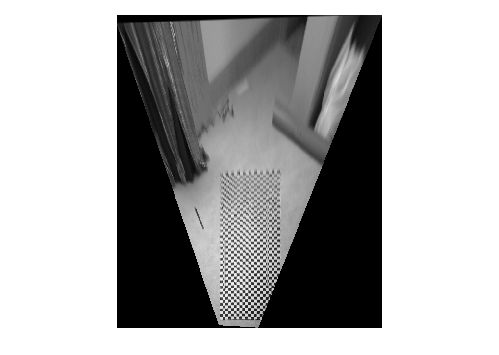
truncate the resulting transformation. We used the previous plot to select the XData and YData limits.

xf2 = imtransform(img,tf,'XData', [ -500 1500],'YData',[-3200 1200]);
imshow(xf2)
imwrite(xf2,[name '_truncated.jpg']);
warning('on',msgid);

Published with MATLAB® R2014a