Ortho

Produce orthonormal view from oblique projective image

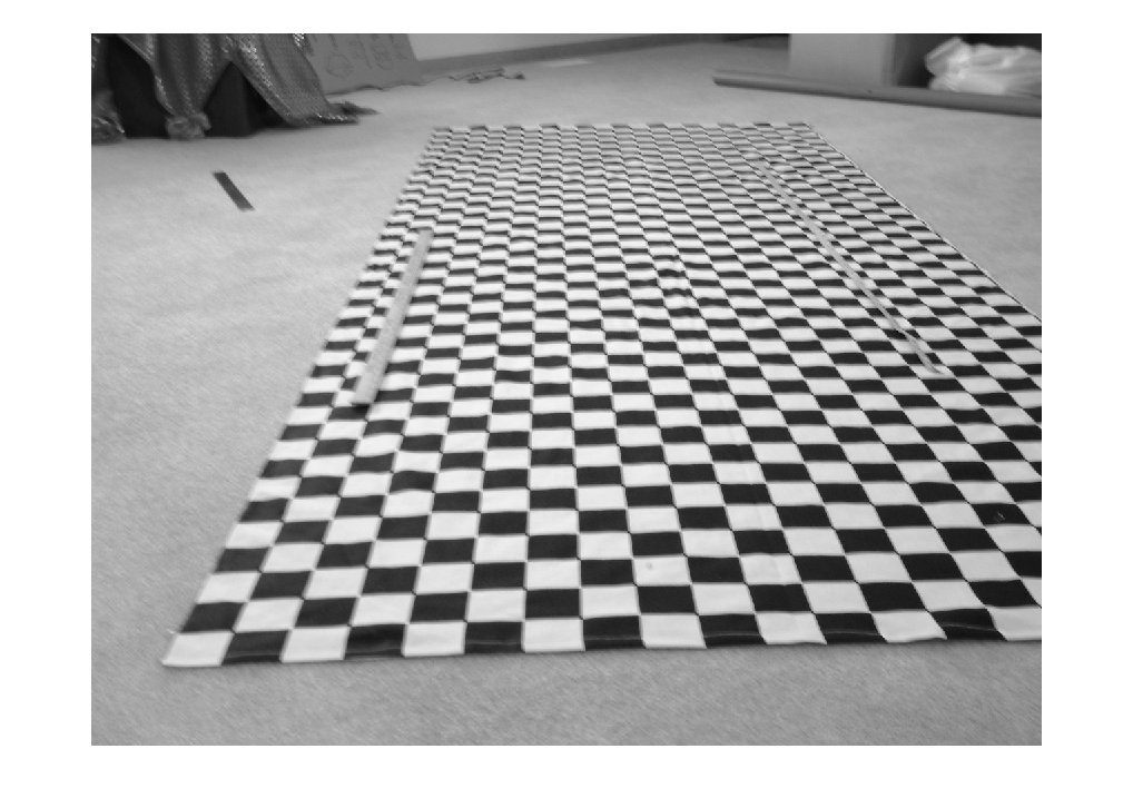
read original image

clear; close all
filename = '2002_1229_125739AA.JPG';
img = im2double(rgb2gray(imread(filename)));
name = 'check2';
msgid = 'Images:initSize:adjustingMag';
warning('off',msgid);
imshow(img);

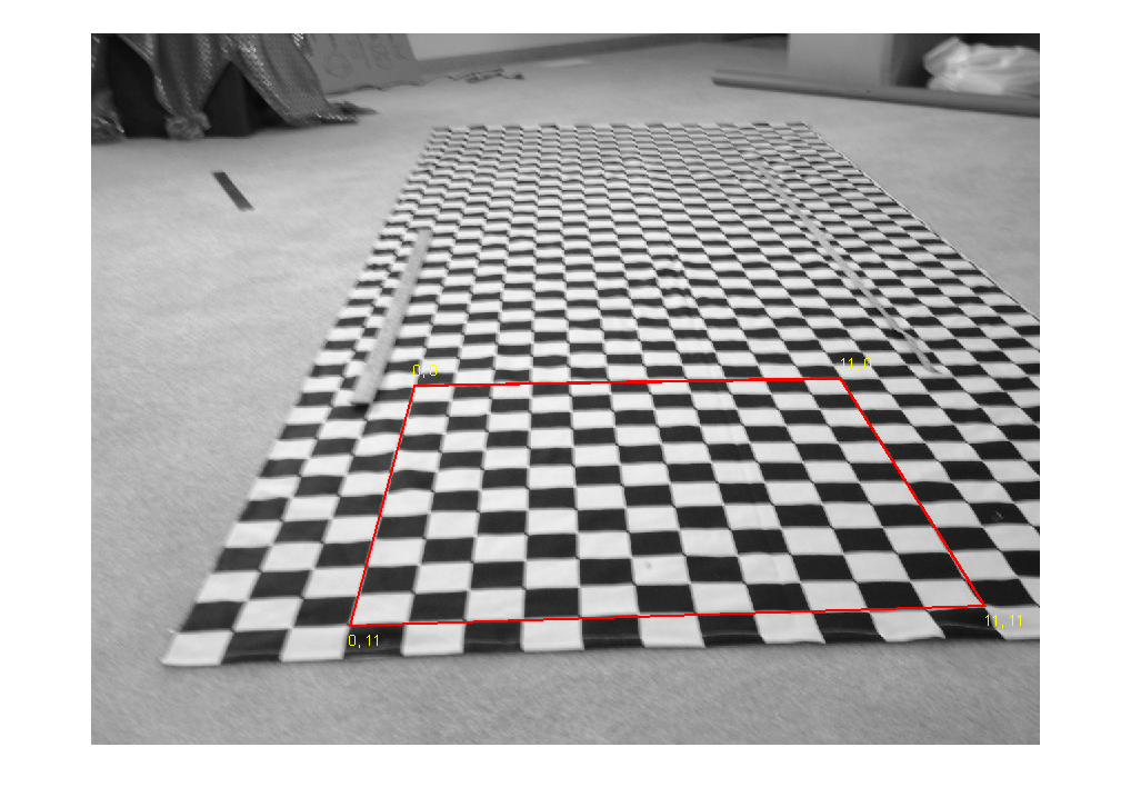
input corners (using impixel) and compute transform

%[c r p] = impixel;
c = [ 349 1207 1012 436 ]';
r = [ 800  773  466 476 ]';
base = [0 11; 11 11; 11 0; 0 0];
tf = fitgeotrans([c r],base*80,'projective');
disp('tf = ');
disp(tf)

tf = 
  projective2d with properties:

                 T: [3x3 double]
    Dimensionality: 2

T = tf.T;
disp('T =');
format short g
disp(T);
format

T =
       5.5216      0.26275  -6.2929e-05
       1.4827       15.135    0.0057103
      -3113.2      -7318.6            1

overlay control points on image

imshow(img);
hold on;
plot([c;c(1)],[r;r(1)],'r','Linewidth',2);
text(c(1),r(1)+20,'0, 11','Color','y');
text(c(2),r(2)+20,'11, 11','Color','y');
text(c(3),r(3)-20,'11, 0','Color','y');
text(c(4),r(4)-20,'0, 0','Color','y');
hold off;
F = getframe();
g = frame2im(F);
imwrite(g,[name '_overlay.jpg']);

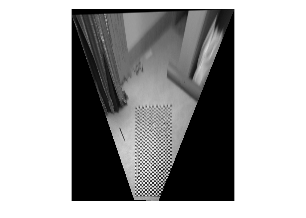
do image transform

[xf1, xf1_ref] = imwarp(img,tf);
imshow(xf1)
xf1_ref
imwrite(xf1,[name '_registered.jpg']);

xf1_ref = 

  imref2d with properties:

           XWorldLimits: [-3.1012e+03 4.2918e+03]
           YWorldLimits: [-7.5629e+03 1.1801e+03]
              ImageSize: [8743 7393]
    PixelExtentInWorldX: 1
    PixelExtentInWorldY: 1
    ImageExtentInWorldX: 7393
    ImageExtentInWorldY: 8743
       XIntrinsicLimits: [0.5000 7.3935e+03]
       YIntrinsicLimits: [0.5000 8.7435e+03]

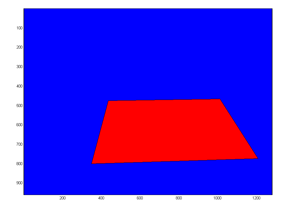
show a simplified form of the original image

bdi = [1 1; 1280 1; 1280 960; 1 960];
fill(bdi(:,1),bdi(:,2),'b');
axis ij;
hold on
fill(c,r,'r');
hold off
axis equal

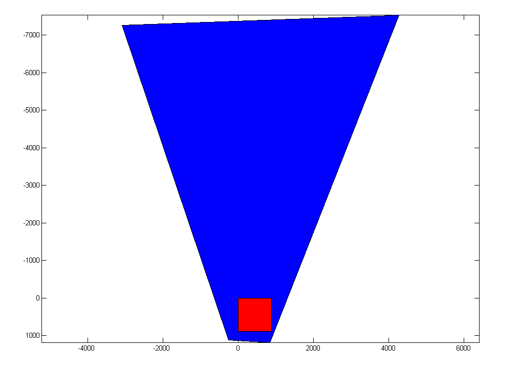
% show the transformed simplified image
rd = transformPointsForward(tf,[c r]);
bds = transformPointsForward(tf,bdi);
fill(bds(:,1),bds(:,2),'b')
axis ij
hold on
fill(rd(:,1),rd(:,2),'r')
axis equal
hold off

% show that the control points map to the target points
prd = [c r ones(4,1)]*T;
% B = repmat(A,M,N) creates a large matrix B consisting of an M-by-N
%     tiling of copies of A.
%  This is used to produce two copies of the the third, homogeneous
%  variable. The end result is to convert homogeneous to normal variables.
uv = prd(:,1:2)./repmat(prd(:,3),1,2);
disp('uv/80 = ');
disp(uv/80)

uv/80 = 
         0   11.0000
   11.0000   11.0000
   11.0000    0.0000
    0.0000    0.0000

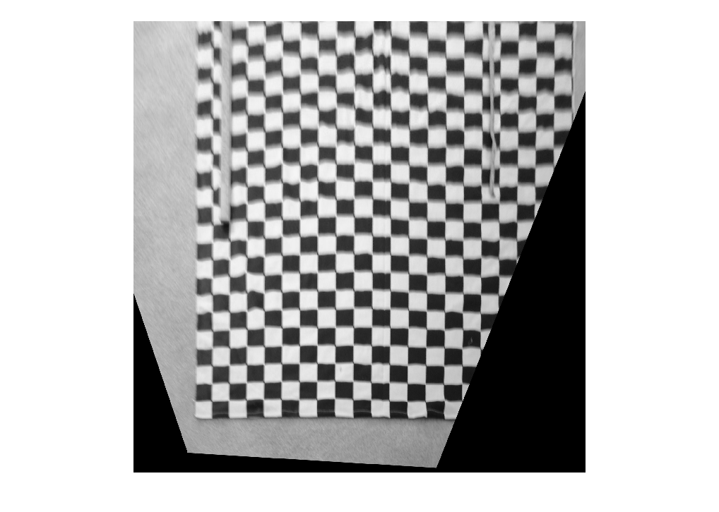
truncate the resulting transformation. We used the previous plot to select the XData and YData limits.

xf1_ref.XWorldLimits = [-500 1500];
xf1_ref.YWorldLimits = [-800 1200];
xf1_ref.ImageSize = [2000 2000];
[xf2 xf2_ref] = imwarp(img,tf,'OutputView',xf1_ref);
xf2_ref
imshow(xf2)
imwrite(xf2,[name '_truncated.jpg']);
warning('on',msgid);

xf2_ref = 

  imref2d with properties:

           XWorldLimits: [-500 1500]
           YWorldLimits: [-800 1200]
              ImageSize: [2000 2000]
    PixelExtentInWorldX: 1
    PixelExtentInWorldY: 1
    ImageExtentInWorldX: 2000
    ImageExtentInWorldY: 2000
       XIntrinsicLimits: [0.5000 2.0005e+03]
       YIntrinsicLimits: [0.5000 2.0005e+03]

Published with MATLAB® R2014a