| On this page… |
|---|
Example: Performing a Translation |
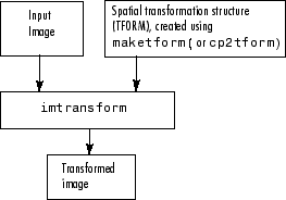
Performing general 2-D spatial transformations is a three-step process:
Define the parameters of the spatial transformation. See Defining the Transformation Data for more information.
Create a transformation structure, called a TFORM structure, that defines the type of transformation you want to perform.
A TFORM is a MATLAB structure that contains all the parameters required to perform a transformation. You can define many types of spatial transformations in a TFORM, including affine transformations, such as translation, scaling, rotation, and shearing, projective transformations, and custom transformations. You use the maketform function to create TFORM structures. For more information, see Creating TFORM Structures. (You can also create a TFORM using the cp2tform function — see Image Registration.
Perform the transformation. To do this, you pass the image to be transformed and the TFORM structure to the imtransform function.
The following figure illustrates this process.
Overview of General 2-D Spatial Transformation Process

This example illustrates how to use the maketform and imtransform functions to perform a 2-D spatial transformation of an image. The example performs a simple affine transformation called a translation. In a translation, you shift an image in coordinate space by adding a specified value to the x- and y-coordinates. The example illustrates the following steps:
Bring the image to be transformed into the MATLAB workspace. This example creates a checkerboard image, using the checkerboard function. By default, checkerboard creates an 80-by-80 pixel image.
cb =
checkerboard; imshow(cb)
Original Image

You must define the spatial transformation that you want to perform. For many types of 2-D spatial transformations, such as affine transformations, you can use a 3-by-3 transformation matrix to specify the transformation. You can also use sets of points in the input and output images to specify the transformation and let maketform create the transformation matrix. For more information, see Defining the Transformation Data.
This example uses the following transformation matrix to define a spatial transformation called a translation.
xform = [ 1 0 0 0 1 0 40 40 1 ]
In this matrix, xform(3,1) specifies the number of pixels to shift the image in the horizontal direction and xform(3,2) specifies the number of pixels to shift the image in the vertical direction.
You use the maketform function to create a TFORM structure. As arguments, you specify the type of transformation you want to perform and the transformation matrix (or set of points) that you created to define the transformation. For more information, see Creating TFORM Structures.
This example calls maketform, specifying 'affine' as the type of transformation, because translation is a type of affine transformation, and xform, the transformation matrix created in step 2.
tform_translate =
maketform('affine',xform);To perform the transformation, call the imtransform function, specifying the image you want to transform and the TFORM structure that stores all the required transformation parameters. For more information, see Performing the Spatial Transformation.
The following example passes to the imtransform function the checkerboard image, created in Step 1, and the TFORM structure created in Step 3. imtransform returns the transformed image.
[cb_trans xdata
ydata]= imtransform(cb, tform_translate);
The example includes two optional output arguments: xdata and ydata. These arguments return the location of the output image in output coordinate space. xdata contains the x-coordinates of the pixels at the corners of the output image. ydata contains the y-coordinates of these same pixels.
Note This section uses the spatial coordinate system when referring to pixel locations. In the spatial coordinates system, the x- and y-coordinates specify the center of the pixel. For more information about the distinction between spatial coordinates and pixel coordinates, see MATLAB documenentation on Image Coordinate Systems. |
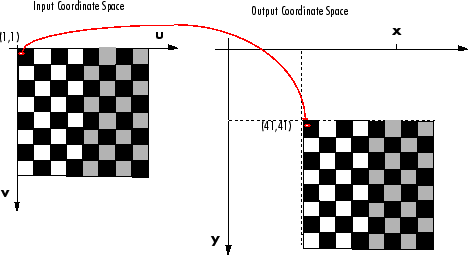
The following figure illustrates this translation graphically. By convention, the axes in input space are labeled u and v and the axes in output space are labelled x and y. In the figure, note how imtransform modifies the spatial coordinates that define the locations of pixels in the input image. The pixel at (1,1) is now positioned at (41,41). (In the checkerboard image, each black, white, and gray square is 10 pixels high and 10 pixels wide.)
Input Image Translated

Pixel Values and Pixel Locations. The previous figure shows how imtransform changes the locations of pixels between input space and output space. The pixel located at (1,1) in the input image is now located at (41,41) in the output image. Note, however, that the value at that pixel location has not changed. Pixel (1,1) in the input image is black and so is pixel (41,41) in the output image.
imtransform determines the value of pixels in the output image by mapping the new locations back to the corresponding locations in the input image (inverse mapping). In a translation, because the size and orientation of the output image is the same as the input image, this is a one to one mapping of pixel values to new locations. For other types of transformations, such as scaling or rotation, imtransform interpolates within the input image to compute the output pixel value. See imtransform for more information about supported interpolation methods.
After performing the transformation, you might want to view the transformed image. The example uses the imshow function to display the transformed image.
figure, imshow(cb_trans)
Translated Image

Understanding the Display of the Transformed Image. When viewing the transformed image, especially for a translation operation, it might appear that the transformation had no effect. The transformed image looks identical to the original image. However, if you check the xdata and ydata values returned by imtransform, you can see that the spatial coordinates have changed. The upper left corner of the input image with spatial coordinates (1,1) is now (41,41). The lower right corner of the input image with spatial coordinates (80,80) is now (120,120). The value 40 has been added to each, as expected.
xdata =

    41   120

ydata =

    41   120
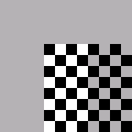
The reason that no change is apparent in the visualization is because imtransform sizes the output image to be just large enough to contain the entire transformed image but not the entire output coordinate space. To see the effect of the translation in relation to the original image, you can use several optional input parameters that specify the size of output image and how much of the output space is included in the output image.
The example uses two of these optional input parameters, XData and YData, to specify how much of the output coordinate space to include in the output image. The example sets the XData and YData to include the origin of the original image and be large enough to contain the entire translated image.
Note All the pixels that are now in the output image that do not correspond to locations in the input image are black. imtransform assigns a value, called a fill value, to these pixels. This example uses the default fill value but you can specify a different one — see Specifying Fill Values. |
cb_trans2 = imtransform(cb, tform_translate,...
                        'XData', [1 (size(cb,2)+ xform(3,1))],...
                        'YData', [1 (size(cb,1)+ xform(3,2))]);
figure, imshow(cb_trans2)
View of the Translated Image in Relation to Original Coordinate Space
Before you can perform a spatial transformation, you must first define the parameters of the transformation. The following sections describe two ways you can define a spatial transformation.
With either method, you pass the result to the maketform function to create the TFORM structure required by imtransform.
The maketform function can accept transformation matrices of various sizes for N-D transformations. Because imtransform only performs 2-D transformations, you can only specify 3-by-3 transformation matrices.
For example, you can use a 3-by-3 matrix to specify any of the affine transformations. For affine transformations, the last column must contain 0 0 1 ([zeros(N,1); 1]). You can specify a 3-by-2 matrix. In this case, imtransform automatically adds this third column.
The following table lists the affine transformations you can perform with imtransform along with the transformation matrix used to define them. You can combine multiple affine transformations into a single matrix.
Affine Transform | Example | Transformation Matrix | |
|---|---|---|---|
Translation | | | tx specifies the displacement along the x axis ty specifies the displacement along the y axis. |
Scale | | | sx specifies the scale factor along the x axis sy specifies the scale factor along the y axis. |
Shear | | | shx specifies the shear factor along the x axis shy specifies the shear factor along the y axis. |
Rotation | | | q specifies the angle of rotation. |
Instead of specifying a transformation matrix, you optionally use sets of points to specify a transformation and let maketform infer the transformation matrix.
To do this for an affine transformation, you must pick three non-collinear points in the input image and in the output image. (The points form a triangle.) For a projective transformation, you must pick four points. (The points form a quadrilateral.)
This example picks three points in the input image and three points in the output image created by the translation performed in Example: Performing a Translation. The example passes these points to maketform and lets maketform infer the transformation matrix. The three points mark three corners of one of the checkerboard squares in the input image and the same square in the output image.
   in_points = [11 11;21 11; 21 21]

   out_points = [51 51;61 51;61 61]

   tform2 = maketform('affine',inpts,outpts)
After defining the transformation data (Defining the Transformation Data), you must create a TFORM structure to specify the spatial transformation. You use the maketform function to create a TFORM structure. You pass the TFORM structure to the imtransform to perform the transformation. (You can also create a TFORM using the cp2tform function. For more information, see Image Registration.)
The example creates a TFORM structure that specifies the parameters necessary for the translation operation.
tform_translate = maketform('affine',xform)
To create a TFORM you must specify the type of transformation you want to perform and pass in the transformation data. The example specifies 'affine' as the transformation type because translation is an affine transformation but maketform also supports projective transformations. In addition, by using the custom and composite options you can specify a virtually limitless variety of spatial transformations to be used with imtransform. The following table lists the transformation types supported by maketform.
Transformation Type | Description |
|---|---|
'affine' | Transformation that can include translation, rotation, scaling, and shearing. Straight lines remain straight, and parallel lines remain parallel, but rectangles might become parallelograms. |
'projective' | Transformation in which straight lines remain straight but parallel lines converge toward vanishing points. (The vanishing points can fall inside or outside the image -- even at infinity.) |
'box' | Special case of an affine transformation where each dimension is shifted and scaled independently. |
'custom' | User-defined transformation, providing the forward and/or inverse functions that are called by imtransform. |
'composite' | Composition of two or more transformations. |
Once you specify the transformation in a TFORM struct, you can perform the transformation by calling imtransform. The imtransform function performs the specified transformation on the coordinates of the input image and creates an output image.
The translation example called imtransform to perform the transformation, passing it the image to be transformed and the TFORM structure. imtransform returns the transformed image.
cb_trans = imtransform(cb,tform_translate);
imtransform supports several optional input parameters that you can use to control various aspects of the transformation such as the size of the output image and the fill value used. To see an example of using the XData and YData input parameters, see Example: Performing Image Registration. For more information about specifying fill values, see Specifying Fill Values.
When you perform a transformation, there are often pixels in the output image that are not part of the original input image. These pixels must be assigned some value, called a fill value. By default, imtransform sets these pixels to zero and they are displayed as black. Using the FillValues parameter with the imtransform function, you can specify a different color.
Grayscale Images. If the image being transformed is a grayscale image, you must specify a scalar value that specifies a shade of gray.
For example, in Step 5: View the Output Image, where the example displays the translated checkerboard image in relation to the original coordinate space, you can specify a fill value that matches the color of the gray squares, rather than the default black color.
cb_fill = imtransform(cb, tform_translate,...
      'XData', [1 (size(cb,2)+xform(3,1))],...
      'YData', [1 (size(cb,1)+xform(3,2))],...
      'FillValues', .7 );
figure, imshow(cb_fill)
Translated Image with Gray Fill Value

RGB Images. If the image being transformed is an RGB image, you can use either a scalar value or a 1-by-3 vector. If you specify a scalar, imtransform uses that shade of gray for each plane of the RGB image. If you specify a 1-by-3 vector, imtransform interprets the values as an RGB color value.
For example, this code translates an RGB image, specifying an RGB color value as the fill value. The example specifies one of the light green values in the image as the fill value.
rgb = imread('onion.png');
xform = [ 1 0 0 0 1 0 40 40 1 ]
tform_translate = maketform('affine',xform);
cb_rgb = imtransform(rgb,tform_translate,...
    'XData', [1 (size(rgb,2)+xform(3,1))],...
    'YData', [1 (size(rgb,1)+xform(3,2))],...
    'FillValues', [187;192;57]);
figure, imshow(cb_rgb)
Translated RGB Image with Color Fill Value

If you are transforming multiple RGB images, you can specify different fill values for each RGB image. For example, if you want to transform a series of 10 RGB images, a 4-D array with dimensions 200-by-200-by-3-by-10, you have several options. You can specify a single scalar value and use a grayscale fill value for each RGB image. You can also specify a 1-by-3 vector to use a single color value for all the RGB images in the series. To use a different color fill value for each RGB image in the series, specify a 3-by-10 array containing RGB color values.
Maintained by John Loomis, last updated 21 February 2011