
Nodal analysis solves for a set of unknown node voltages by using a set of Kirchhoff current law equations (KCL), representing the sum of currents leaving a node, in terms of the node voltages. One node is designated the reference node (assumed to be zero voltage) and is not included in the set of equations.
Consider the resistor below. Positive current leaves node i and negative current leaves node j.
For example, if a conductance GN connects from node i to node j then the terms shown in the figure below appear in the KCL equations.
We can construct a conductance matrix Gm, initially set to zeros, and for each new conductance we can update the conductance matrix according to the template below.

If TN is the template matrix, then the update is represented by
Current sources appear in the KCL equations as entries into the right-hand side excitation vector. A current having direction from node i to node j accumulates positively for KCL for node j and negatively for KCL on node i. The diagram below identifies i as the from node for positive current and j as the to node for positive current.
A MATLAB function for current sources is given in srcAcc.m.
The example below shows two resistors in series with an independent current source. The KCL equations for nodes 1 and 2 are shown next to the circuit.
 | 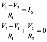
|
The equations can be written in matrix form as
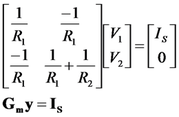
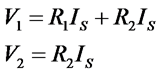
The solution y = Gm \ Is, could be obtained directly from the Kirchoff Voltage Law (KVL) equations:
Example MATLAB code shows the setup and solution of this circuit using both symbolic and numeric functions. See results.
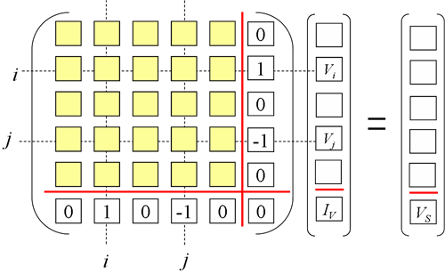

For node i: Gm V + IV = 0
For node j: Gm V − IV = 0
Additional equation: Vi − Vj = VS
See results.
Maintained by John Loomis, last updated 6 March 2009