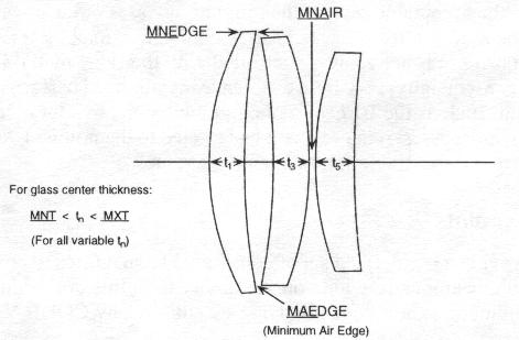
Figure 2. General Constraints on element thickness and spacings.
The AUTOMATIC DESIGN option or (AUTO) is aimed at changing the lens system to improve its performance, in fact to achieve the best possible performance subject to the constraints on the system; the changed lens becomes the lens data base as if it had been entered in the LDM for any future analyses or operations. The uses of AUTO can range from the simple to the complex:
The AUTO option is also driven by the options:
These options have inputs of their own, then enter AUTO to do the optimization according to the constraints and performance measure commands defined here. See TES or CAM options (Chapter 7) for details.
Any list of uses, even a detailed list, would be hopelessly incomplete. The essence of the AUTO option is that it is a way of changing all of the permitted variables in a lens simultaneously so that the lens is improved in the sense defined by the performance measure, yet holding fixed other requirements (the constraints). Other than the simplest cases, it is a process that is impossible to do by "hand" - user-selected changes in the permitted variables.
The variables (parameters allowed to change during optimization) are declared in the LDM by using the control codes to freeze, vary, or couple the corresponding parameters. User-defined apertures are not used; only the vignetting factors from the LDM are used to declare pupil shape at each field (except in MTF optimization which uses apertures and obstructions). Gaussian apodization and any user~efined-apodization (INT) that is applied to the entrance pupil is used as part of the aperture weighting for the error function; surface-based apodization and polarization is ignored. LDM wavelength weights are used unless overridden by a WTW local to AUT.
The design of a system is seldom accomplished by one AUTO run. You are part of a process which allows you to start with a tentative lens system, impose obvious constraints, and optimize the lens to a default performance measure; inspection of the results, as evaluated by any of the other CODE V options, will guide you to change one or more of the following:
Subsequent runs will continue the process toward achieving the desired lens system. Much of the activity of lens design is associated with becoming adept at correlating results of optimization runs with the changes needed in these four areas to provide the "best" solution for your project.
Note that the AUTO option can only solve the problem you give it.
It cannot:
Once you have selected the starting point lens and defined it in the LDM, there are three fundamental areas in which you will supply inputs that will drive the action of the AUTO option:
A very simple, but possibly very useful, run that includes an optimization may consist of commands like the following:
RES CV_LENS: TRIPLET ! Restore one of the standard CODE V lenses
DEF VAR S1..I        ! Set up the default variable set on all surfaces
AUTO                 ! Enter the AUTO option
EFL = 100            ! Constrain the effective focal length to 100
GO                   ! Begins the optimization
SAV MYLENSOPT        ! Save the lens after optimizing it
An important key to using the optimization effectively is a good understanding of how constraints are handled by AUTO. The standard method of constraint control used in CODE V is called the Lagrangian Multiplier method. This method has a number of advantages:
When a constraint is active, it is imposed as an absolute condition on the solution and thus can have a rather major effect on the rate and smoothness of convergence as well as on the quality of the optimized lens. In general it is good practice to impose the fewest constraints possible, particularly in the early stages of a design. Never use a constraint to impose a condition that is already represented in a solve; for example, do not use both an OAL solve and also an OAL constraint, both of which provide the same control. If they both were to be imposed for the same interval of surfaces, a singular constraint condition would be generated, which is to be avoided, even though the "smart equation solver" in CODE V would detect the condition and ignore the constraint.
Specific constraints are those which you specify either as target values, or one-sided boundaries; the entry of two boundaries can define a range of acceptable values. Specific constraints can be:
Constraint targets are defined in command mode using the = sign, as in EFL = 100; boundaries are defined using the < and/or > symbols, as in IMD > 25.8. Both limits of a range may be entered in the same command as in:
IMD > 28 < 35 ! Image distance must be between 28 and 35 lens units
When defining a range or a boundary, it is possible for the actual value of the quantity constrained to lie within the range or on the acceptable side of the boundary. In this case. we say the constraint is "inactive", although the program is monitoring it, to see if it crosses into the unacceptable region, at which point it is activated. Active constraints are also monitored to check the direction the constraint would move if released; if the value would move into the acceptable region, the program releases or deactivates the constraint. This allows the error function to be reduced in the least constrained manner, making for improved convergence. Note that when a bounded constraint is active, it is controlled with the same method and the same precision as is the targeted constraint; consequently, very little difference in optimized performance would be observed between targeting a constraint, such as the EFL of a photographic objective lens, and bounding it between two closely spaced values. In most cases. it may as well be targeted to the nominal value. instead of using up part of the production tolerance by constraining it to a range of values.
It is not possible to provide a pre-defined set of constrainable quantities to cover all possible needs in optical design. User-defined constraints provide you the ability to define constraints specific to your own needs. They can contain arithmetic expressions involving essentially any CODE V database item, and any of the pre-defined constraints. Please refer to the section "User-defined Constraints" in the Technical Notes for this option for more information and examples of user-defined constraints as well as the Reference Manual section on the CODE V macro language called Macro-PLUS; the lens database items, pre-defined quantities, functions and expressions that can be used in user-defined constraints are all documented as part of the Macro-PLUS description (Chapter 11).
Although the default mode is for constraints to be kept separate from the error function, it is possible to include one or more specific constraints in the merit function, by entering the WTC command (along with a weight) after the constraint entry. This should only be done on targeted constraints, not bounded constraints. An example of its use in command mode is:
Y R1 S12 F3 = 0.0 ! Constrain the chief ray, surface 12, field 3 to 0.0
WTC .1            ! control prior constraint with the error function
This mode is useful primarily when the constraint is very non-linear, when the current value of the constraint is a long distance from the target, or when several constraints are in conflict or nearly in conflict with one another. The inclusion in the error function provides a much less rigid control, and one that is less disruptive and more adaptable in such situations.
General constraints differ from specific constraints in almost every aspect. Whereas a specific constraint must be explicitly imposed and only applies to a specific surface and a specific zoom position, the general constraints apply to all surfaces and all zoom positions and (except for MXA) are automatically imposed with default values. The general constraints relating to thicknesses cannot be given different values for different surfaces or different zoom positions; one value is used globally. All general constraints are always imposed as bounds (never as equality constraints) and cannot be included in the error function with WTC (they are always controlled with the method of Lagrangian multipliers). A general constraint on a specific surface and zoom position is overridden by a corresponding specific constraint applied to that surface and zoom position; the general constraints remain imposed on all the other surfaces.
There are seven general constraints. Five of them control element thicknesses and spacings (MXT, MNT,MNE.MNA, and MAE), one controls the movement of variable glasses (GLA), and one controls maximum ray angle of incidence (MXA). All except MXA are imposed automatically with program generated default values which you can override.
The five general constraints relating to element thickness and spacing (MXT,MNT,MNE,MNA, and MAE) are shown in Figure 2. The default values for center thickness (MXT and MNT) and edge thickness (MNE) are a function of the scale of the lens. The default values on air spacing at the axis and at clear apertures (MNA and MAE) are fixed with the lens dimensions (inches, mm, or cm). The general constraints relating to center and edge thickness can be overridden for a specific surface and zoom position by the entry of a specific CT or ET constraint for that surface and zoom position; this will disable all other general thickness constraints on that surface for all zoom positions. Note that these five general constraints can only be controlled if the appropriate thicknesses are variable. If the thickness is frozen, general thickness constraint violations can occur.
Figure 2. General Constraints on element thickness and spacings.
On any given surface there can be only one active general thickness constraint. If on a given surface more than one of the general thickness constraints is in violation, AUTO selects the one with the largest violation and controls it for that cycle (it may release it and control a different one on the next cycle). In a zoomed system this same technique is used, although it may not be sufficient in all cases. In a "true zoom" system, this technique is sufficient to control all the general thickness constraints. However, in a general zoom system, or multi-configuration system, this technique may not be sufficient and it may be necessary for you to enter specific CT and/or ET constraints as a function of zoom position (remember that entering either CT or ET specific constraints in any zoom position disables all the general thickness constraints for all zoom positions on that surface).
The general constraint relating to variable glasses (GLA) is automatically imposed on surfaces with variable glasses (see Chapter 2A, "Entering/Changing Data - Materials - Using Fictitious Glasses"). The default constraint is imposed on all such surfaces, although you can override the default constraint on any or all such surfaces (the GLA constraint accepts a surface qualifier). The constraint takes the form of a three to five-sided convex polygon drawn on a plot of N vs. AN. It is best to make the corners of the polygon equate to real glasses (this is the default case). Note that the default constraint corners correspond to Schott glasses; if you are using other catalogs, you may wish to change the default values appropriately. If any of your fictitious glasses have a partial dispersion setting (GDP command in the LDM), then you will want to specify an appropriate GLA constraint for that surface to limit its motion to the range valid for that anomalous dispersion glass family (see Chapter 2A, "Entering/Changing Data - Materials - Dispersion of Fictitious Glasses").
The general constraint on reference ray angle of incidence (MXA) improves the efficiency of Global Synthesis runs by eliminating regions where solutions are less likely to be found; it can be used in non-GS runs as well. MXA specifies the maximum angle of incidence (or refraction) on the surface for all active reference rays (rays listed by RSP). The value specified is the maximum angle in degrees from the surface normal at the point of intersection with the surface on the side with the lower (absolute value of) refractive index. The default is MXA NO, meaning the constraint is not imposed. MXA YES with no value enters a default value of 60�. When MXA is imposed by you, it can be imposed on all surfaces or on a surface range (MXA accepts a surface qualifier). The allowable surface range is S l..I- 1, which is also the default surface range (SA is not allowed, since it means S0..I).
MXA commands are cumulative; successive MXA commands can enter different values for different surfaces or ranges of surfaces. On NSS surfaces which can be hit more than once, MXA only constrains the last hit (such surfaces should be excluded from the MXA surface range). The MXA constraint for a specific surface is overridden by explicit AOI or AOR constraints on that surface.
You are strongly urged to review the information in the command summaries of constraints because much of the information regarding the use of particular constraints is given there. Some additional information on various constraints, and their interactions is given below:
As mentioned above in the discussion of general constraints, CODE V sets up default constraints for the control of center and edge thicknesses. It is important to understand how these interact with each other and with the specific CT and ET constraints. If a value for the MXT (maximum center thickness) constraint is specified such that it is in conflict with the MNT (minimum center thickness) or MNE (minimum edge thickness) constraint, the program ignores the MXT constraint and automatically ensures that the MNT or MNE constraints are imposed (the program imposes MNT or MNE depending on surface shape). Similarly, any frozen thickness removes the general thickness constraints, allowing powers to be distributed optimally without regard to edge thickness. Thus, in both cases, the natural inclinations of the system for distribution of power on the surfaces are conveyed to you rather than being distorted by the requirements to satisfy these conflicting conditions. This becomes a particularly useful feature when system requirements (such as minimum weight) require that elements be kept thin; in this case an artificially small MXT value can be specified which will have the effect of keeping all of the element thicknesses just large enough to satisfy the MNT or MNE values. If, however, you wish to impose absolute conditions on the maximum center thickness and the minimum edge thickness for one or more elements, this can be done by specifying CT and ET values for the surface or surfaces in question. The entry of a CT or ET value for a surface (or IMD, IMC for image clearance) will always completely deactivate the general center/edge thickness constraints for the surface.
The classical distortion calculation is typically applicable only for centered and rotationally symmetric systems. In this case the field should be specified with Y components only, and the DIY distortion control is the appropriate one to use. The distortion is calculated by differencing the paraxial image height and the actual chief ray image height and then dividing by the paraxial image height. In the presence of defocusing or non-flat image surfaces, the chief ray is extended to intersect the flat paraxial image surface and that value is used as the chief ray image height in the distortion calculation. DIX can be used for anamorphic systems when XZF (LDM) is set to get the X-plane EFL value used in the calculation and the reference Fk has an X component.
Folded systems and unobscured reflecting systems often pose challenging packaging problems. The ability to control surface and ray data in a global coordinate system is particularly helpful in such cases. The constraints relating to the surface locations (XSC, YSC, ZSC, LSC, MSC, NSC) and those relating to real ray data (X, Y, Z, L, M, N, SRL, SRM, SRN) can all be constrained in a common coordinate system by including the G qualifier identifying the surface number of the coordinate system to use as a global reference. It is sometimes helpful to use user-defined constraints in addition to define the appropriate relationships for a given system. (J. Michael Rodgers, "Control of Packaging Constraints in the Optimization of Unobscured Reflective Systems," SPIE Proc. 751, pp. 143-149. If you are interested in the subject of constraining mirror systems to be unobscuring, please request a copy of the referenced paper from ORA).
It is possible to design lenses that are very sensitive to fabrication errors. It can then become important to reduce the sensitivity of the design to these errors, especially for lenses which are to be produced in quantity by methods designed to lower costs.
The technique used here (SNS) is the sensitivity to tilting of the optical surface (see H. H. Hopkins and J. J. Tiziani, Brit. J. Appl. Phys., 17, 33 (1966) and D.S. Crey, Applied Optics, 9, 523 [1970]). This technique only calculates the tendency to introduce decentered (axial) coma but, for many systems, will adequately represent the sensitivity to decentering over the field. The value listed out is the square root of the variance of the wavefront produced by a radian angular tilt of the surface, measured in the system units. Real tilts are, of course, much smaller and the values may be scaled down by the angle in radians. Thus to convert to waves of aberration
where
| a | is the angle in radians |
| S | is the listed value of the square root of the variance |
| l | is the wavelength in lens system units |
For spherical surfaces, if it is desirable to change the interpretation from tilt sensitivity to displacement sensitivity, multiply each value by the curvature of the surface. Thus the displacement sensitivity is
where d is the displacement in system units and r is the curvature of the surface.
In AUTO, these sensitivity values are derived only from the R2 reference ray on axis and are suitable as constraints to limit or reduce sensitivities. They are unsuited for detailed tolerancing except in the roughest sense; use the tolerance options of CODE V (TOR and TOL) for this.
The optimization in CODE V is primarily based on real ray tracing (although third-order aberrations can be included if desired). This avoids the limitations of aberration theory (third-, fifth-, ... order) when dealing with high aperture and wide angle lenses. A major limitation of the use of aberration theory in optimization is that, during the course of design, the targets are continuously moving as different balances become optimum; this is because the specific aberrations are rarely a direct measure of performance. Another reason for the dependence on ray tracing is that tilted/decentered systems, unusual surface shapes, and variations of the aberrations with wavelength can be precisely modelled; the effects of vignetting and obscurations can be simulated more realistically as well.
The computer "sees" lens quality in terms of the error function (sometimes referred to as a merit function, although it is really a demerit function). This error function is a single positive number which is a composite of all the image errors, appropriately weighted, and may or may not include various constraint deviations (optical, packaging, etc.). The ideal lens would have an error function value of zero, meaning no image errors of any kind. In most cases the error function value will be non-zero, and the function of optimization is to reduce this error function to its minimum possible value, subject to the limitations of the constraints imposed.
The degree to which experienced designers will agree with the quality criterion obtained by the computer for a given design depends on the construction of the error function, and upon the weightings and targets of the components of the error function. In general, the error function construction will be different for different lens design tasks, just as the performance specifications and constraints are different for different lens designs. Since the error function is such a critical part of design and optimization, many designers spend a great deal of effort and time constructing the error function and defining the component aberrations, and their corresponding targets and weights, which make up the error function.
Fortunately, for most designs the choice of error function is neither extremely delicate nor very difficult with the approach embodied in CODE V. A default error function with defaulted but overrideable weightings is used. This has been proven to be a powerful error function on thousands of different lens designs. However, for the more demanding or unusual lens configurations, or for the designer who desires more control over the error function construction, more power and flexibility is available to enhance the error function as needed, but at the expense of more designer time and effort. In CODE V there are four basic ways to define the error function; in most cases the first, or default, method will be sufficient. The choice of error function is controlled by the ERR command. In all four types of error functions the usage of constraints is the same. The four types of error function are:
The default error function is based on the weighted transverse ray aberrations for a rectangularly spaced grid (in the entrance pupil) of rays traced at each non-zero-weighted wavelength. The ray grid is determined by the value of DEL, which defines the ray spacing in a pupil of normalized radius 1; thus, both the number of rays in the grid and the location of the grid relative to the pupil boundary is determined by the particular value of DEL chosen. The default value of DEL (0.385) provides a 12 ray pattern in the half pupil with the outermost rays in the grid Iying nearly at the edge of the pupil (Figure 3).
No. Radius DEL of Ravs at Min DEL Rav Pattern 1.414213 - 0.632456 2 0.447214 0.632455 - 0.471405 6 0.745357 0.471404 - 0.392233 8 0.832052 0.392232 - 0.342998 12 0.874477 0.342997 - 0.282843 16 0.824622 0.282842 - 0.262613 22 0.928477 0.262612 - 0.232496 26 0.885318 0.232495 - 0.220864 30 0 949972 0.220863 - 0.210819 34 0.954524 0.210818 - 0.202031 38 0.958317 0.202030 - 0.194258 40 0.961528 0.194257 - 0.181072 44 0.932125 0.181071 - 0.175412 48 0.968744 0.175411 - 0.165522 56 0.943621 0.165521 - 0.157135 60 0.949335 0.157134 - 0.153393 62 0.976187 0.153392 - 0.149907 70 0.977274 0.149906 - 0.143592 74 0.957878 0.143591 - 0.140720 78 0.980001 0.140719 - 0.135458 82 0.962610 0.135457 - 0.133039 86 0.982149 0.133038 - 0.130745 90 0.982764 0.130744 - 0.128565 94 0.983333 0.128564 - 0.126492 96 0.983877 0.126491 - 0.120825 104 0.955205 0.120824 - 0.117445 108 0.972030 0.117445 - 0.115857 116 0.986487 0.115856 - 0.114333 120 0.986847 0.114332 - 0.112867 124 0.987183 0.112866 - 0.108786 128 0.963846 0.108785 - 0.107521 134 0.988375 0.107520 - 0.105400 138 0.980277 | 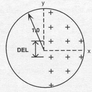
|
Figure 3. Ray pattern in the entrance pupil.
AUTO only includes those rays in the pattern which are not redundant; thus, in a symmetrical system on axis, the default pattern is an octant containing 4 rays, appropriately weighted to represent the full pattern. Off-axis, if the system has bi-lateral symmetry, only one-half of the pupil needs to be represented; in the presence of non-rotationally symmetric surfaces, tilts or de enters out of the Y-Z plane, or X components in the specification of the field points, rays are traced in the full pupil, which approximately doubles the computing time. Ray grids in non-reference wavelengths are traced to the same entrance pupil as the reference wavelength unless specified otherwise (CPA).
The effect of vignetting on the ray pattern is to scale down the portion of the ray grid pattern to which the vignetting applies, instead of clipping rays out of the pattern based on the amount of vignetting specified. This approach was chosen to keep the error function a mathematically continuous function as the vignetting is changed, rather than a step function. Note that any apertures that may have been entered for the lens in the LDM are not considered in defining the ray grid pattern.
In addition to symmetry considerations, the vignetting and the value of the ray interval (DEL), the only other inputs that affect the ray grid pattern are OBS (to obscure a central fraction of the aperture), MER (to collapse the pattern on to the meridional plane), SAG (to collapse the pattern on to the sagittal plane), and SAP (to produce a grid extended out to fill a square entrance pupil instead of a round one).
The default error function is made up from transverse ray aberrations, which are the deviations of the rays in the various grids from their respective reference wavelength chief ray (refer to the section on Construction of the Error Function). In some instances deviations from the image centroid is more appropriate. This can be done with the CEN command. (Refer also to the constraints on image centroid, XCN and YCN.) Note that using CEN will tend to allow more coma in the image.
While using the default error function can produce excellent designs in some cases, it is usually worthwhile to experiment with changing the weights and controls affecting the error function construction before completing any given design task, because the improvement in performance achieved or balance between fields can sometimes be quite dramatic.
The alteration of default DEL and weights should be done with the following context in mind:
The value of DEL (which affects the number and placement of rays in the ray grid) is one of the more important parameters affecting the error function that can be modified; some suggestions and reasons to modify it are:
You can also use both X and Y vignetting to artificially shrink or expand the grid during AUT, restoring it afterwards for evaluation; just be sure the lens sizes are sufficient to pass the bundles for analysis.
The performance specification for a lens is often given in terms of the diffraction MTF at specified spatial frequencies and azimuths for specified field points. Use of an error function based on mean square spot size or wave aberration to achieve these MTF goals frequently requires considerable designer interaction. Using the CODE V default error function to accomplish this often involves multiple AUTO runs, varying the DEL and WTA parameters to achieve the MTF goals. The MTF optimization capability in CODE V provides an effective way of optimizing MTF directly. This would normally be used during the final stages of a design where final balancing is needed, although it can be used anytime. Transverse ray aberration or wavefront variance (OPD) error functions are more appropriate for the early stages of design both for efficiency and because of the more monotonic variation of the error function with lens parameters. In the later stages of design, when the design isn't changing much, the designer can switch to the MTF based error function. In this mode, unlike the default error function, the user-defined apertures in the lens are taken into account when defining the pupil, including non-circular apertures and obstructions. Note, however, that MTF optimization does not use apodization, either Gaussian or user-entered with .INT files.
The MTF error function is enabled by the input of the FRE command. Other MTF error function commands are ignored unless this command is also giver.. Once the FRE command is given, the standard default error function is replaced with the MTF error function. You cannot optimize using both forms of error function at the same time. Note that centroid constraints (XCN and YCN) cannot be used with MTF optimization. If either is entered, the FRE command is ignored; if the FRE command is entered first, then the XCN and YCN constraints cannot be entered.
The FRE command is used to specify the spatial frequencies at which the MTF will be optimized. Up to six may be defined for each field/zoom position, and they may be different for each field/zoom position (including different numbers of frequencies). The AZI command is used to define the azimuth for each of the spatial frequencies entered with FRE. The quantity which is minimized is the square of the weighted difference between the actual MTF and a target value. The weights are specified with the WTM command. This can be used to shift weights to higher or lower frequencies, or to emphasize certain fields or zoom positions, in order to balance the solution. The default is equal weighting for all frequencies.
The MTF targets are specified with the TGM command; the default is the diffraction limit for each frequency Note that since what is optimized is the square of the difference between the MTF and its target. MTF -'alues above the target as well as below the target are errors. Well chosen target values can significantly improve the convergence. When an optimization run is allowed to progress without user intervention, choosing a target that is too low allows the program to attain the target value, ard then prevents it from further improving the performance. On the other hand, setting a target value that is far away from the current value of MTF may necessitate excessive damping of the solution which impedes the convergence of the run. It may be appropriate to run only a few cycles at a time and reexamine the target values frequently. If the MTF at a particular frequency actually attains its target value, then one should either increase the target or, in some cases, delete that spatial frequency from the error function.
Sometimes it is appropriate to include the phase transfer function in the error function, such as when trying to emphasize symmetry in the image. This can be done with the WTP command, which defines the relative weighting between the phase transfer function and the MTF. The weight applies to all frequencies and the target for the phase transfer function is always 0.0. A WTP of 0 means ignore the phase entirely and concentrate on meeting the MTF target values. A large value shifts emphasis to holding the phase to 0.0 and deemphasizes meeting the MTF targets.
There are two controls on the grids used for the MTF calculations. NRD is used to set the density of the grid used to determine aperture and obscuration boundaries and to fit the wavefront polynomials. The default value is appropriate for most cases but can be increased for complex aperture shapes and/or severe aberrations. It can also be decreased, when appropriate, to reduce computation time. The DEL value controls the density of the grid used in the calculation of the MTF integrals and can be reduced for more accuracy at the cost of increased computation time. However, it is not always necessary to have as much accuracy in the MTF calculation during optimization as in final evaluation; if the derivatives and location of the minima are modeled correctly then the convergence will be the same.
There are no firm rules for selecting the frequencies at which to optimize, but there are a few guidelines that should be followed for best results. If the lens is not already near its final configuration (and hence the image quality is not very good), it may be advisable to select MTF frequencies lower than those desired, and in subsequent runs move the frequencies up to the desired ones. This can sometimes avoid getting trapped in spurious resolution. Also, it is best not to select too many frequencies for optimization; usually one or at most two frequencies will be sufficient. If optimization over a large frequency range is desired, it may be better to use the standard error function with OPD. It is advisable, however, to put in both radial and tangential azimuths at the selected frequencies. This can be easily done (e.g., FRE 30 30; AZI RAD TAN).
The MTF optimization uses analytic wavefront differentials to compute the derivatives of the OPD with respect to the variables. The technique is identical to that employed in the TOR option. The result is an extremely fast optimization of the diffraction MTF: A typical cycle of MTF optimization will only take about a factor of two longer than a normal optimization cycle. However, often the lens will converge to the result in fewer cycles than needed for the conventional optimization, resulting in less total time needed to achieve the desired MTFs.
Optimizing at multiple image planes may be an effective way to increase the depth of focus of an optical system. One technique to do this would be to zoom the image thickness and perform a multi-configuration optimization with appropriate constraints to keep the image plane separations fixed at the desired locations. The major drawback to this approach (other than using up zoom positions which may be needed for other purposes) is that this requires the program to ray trace each image plane independently, retracing ray grids that are in fact identical for each image plane.
This is not necessary in CODE V. The TFO (through-focus optimization) command provides a method for optimizing one or more configurations (zoom positions) at up to seven focal positions each without the need for extra ray tracing. Invoking the TFO command sets up the specified focal planes for each configuration at which optimization will take place. The locations of these focal planes with respect to the nominal focal plane do not change during AUTO (the locations are not variables), and hence do not need constraints to hold their spacing. Note that only if one of the specified focal planes is at 0.0, will optimization take place at the nominal focal plane. Optimization is done only at the image plane locations specified with the TFO command. AUTO traces rays for the nominally focused system, then appropriately adjusts the ray intercepts and optical path lengths to simultaneously provide equivalent ray trace data at the specified image locations.
Nonsymmetric image plane distributions are easily modeled. The image locations specified with TFO do not have to be uniformly spaced. Different image plane locations can be specified for each field and zoom position, if desired, as well as different numbers of image plane locations. The error function can be weighted by focus position (WTT) or by focus position and field (WTF, WTY, and WTX). A T qualifier is used to denote focus position in these commands.
The through-focus optimization can be used with either the default error function (transverse ray aberration or OPD) or with MTF optimization. Atter the TFO command is entered, error function weights for either optimization mode will accept T qualifiers, with acceptable values according to the number of image locations specified with the TFO command for that field/zoom position.
The ERR command allows user choice of error function types. The default is ERR CDV, which specifies the standard, or default, CODE V error function (using either transverse ray aberrations, OPD, or MTF optimization). In addition to this, the ERR USR command allows definition of a user-defined error function (UDEF) completely of your own design. The UDEF can be composed of predefined aberrations (e.g. X, Y, Z, L,...,DX, DY, etc.), and/or user-defined aberrations specified by single line Macro-PLUS expressions or user-defined Macro-PLUS function calls. In the UDEF. constraints are handled the same way as in the default error function, including use of WTC and Lagrange multiplier constraints. The UDEF can be used by itself or can be used along with the default error function (ERR BTH)
The first step in constructing a UDEF is to define the set of rays to be traced. This can be done with the RAY command, which allows up to four additional reference rays (R6, R7, R8, and R9) to be added to the standard five reference rays at each field and zoom position. These rays must be defined for each desired field which will use them. Another way is with the ENT command; this is the preferred way. The ENT command (for entrance ray) defines the normalized ray coordinates on the entrance pupil (or the vignetted entrance pupil with ENT VIG). or actual coordinates on a selected surface (the ray will be iterated to hit these coordinates). Rays defined with ENT do not have any field associated with them. The aberration ray set is then defined by connecting selected field points with selected rays (ENT or RAY rays) via the ABR command. Unlike the reference rays (RAY). there is no limit to the number of ENT rays that can be defined. ENT LIS will immediately generate a list of all the entered rays and targets along with their ray number (Ek). To modify an ENT ray definition use the E qualifier; do not use the E qualifier when initially entering the ray.
For an example of the entry of ENT rays, consider the ray pattern shown in Figure 4, consisting of five rays along the tangential meridian, two additional rays in the sagittal meridian, and two skew rays. The commands to enter these rays for the vignetted pupil are (note that the chief ray is already defined as reference ray R1):
ENT VIG 0 .95 ! Tangential rays ENT VIG 0 .7 ENT VIG 0 -.7 ENT VIG 0 -.95 ENT VIG .7 0 ! Sagittal rays ENT VIG .95 0 ENT VIG .5 .5 ! Skew rays ENT VIG .5 -.5 | 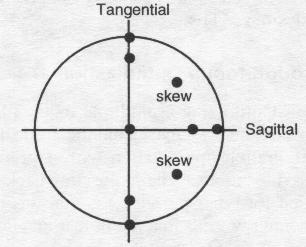
|
Figure 4. Example user-defined ray grid.
When the UDEF is enabled, CODE V maintains a database which keeps track of all the aberration rays (ENT rays) that have been defined, and of all the ray data that is needed to evaluate aberrations specifically requested by you. The ray data is stored in a table so that each aberration ray need only be traced once for each error function evaluation, even if multiple references to the same ray are made with separate ABR commands.
The second step in defining the UDEF is defining the aberrations which will compose the UDEF. This is done with the ABR command (for aberration). The ABR command selects one or more rays (either ENT or RAY rays, selected with E or R qualifiers, respectively) and one or more fields to use these rays, and defines the aberration for those rays. The aberration is selected from a pre-defined list, including ray heights, direction cosines, differences from chief ray, etc. (refer to the ABR command syntax for a complete list). A separate aberration database item (ABR Ak) is defined for each unique combination of ray and field qualifiers on an ABR command. The ABR command also includes the weight of the aberration (default 1.0) and its target value (default 0). If the weight is non-zero (default) the aberration is also entered into the error function calculation. If the weight is zero, then the aberration is only added to the aberration database, but is still accessible to Macro-PLUS. The ABR command is also used to enter a single line Macro-PLUS expression (defined similarly to a user-defined constraint) into the aberration database (and into the error function with non-zero weight).
The use of range qualifiers (..) on fields, rays, wavelengths, surfaces, etc., allow multiple aberrations to be defined with a single ABR command, thus eliminating the need to define a separate name for each aberration. At least one field qualifier (F) and one ray qualifier (R or E) are required (or a user-defined constraint or function); other qualifiers not specified will use default values. Examples of the use of the ABR command are:
ABR F1 E1 DY                     ! Enters one aberration
ABR F1. .3 E1..5 W1. .3 DX       ! Enters 45 aberrations (3 fields X 5 rays X 3 WLs
ABR F2 R1 Y 1.0 33.45            ! Non-zero target
ABR F1 E1 S7 Y 0.3               ! Non-image surface, weight different from unity
ABR @abcd 1 .7                   ! User-defined constraint @abcd targeted to 0.7
The error function in the UDEF uses the aberration targets and weights from the ABR commands and takes the form:
where Ai are the aberration values, Wi are the weights, and Ti are the targets. Within AUTO the aberration values are accessible to Macro-PLUS via the ABR database (ABR Ak), and may be combined with other database items in single and multi-line user-defined function or constraint definitions. These functions may subsequently be used in additional ABR commands to enter user-defined aberrations. Note, however, that CODE V only saves specifically requested aberration data when it traces an aberration ray. Ray data for a given ray that is not requested by one or more ABR commands is discarded, and is not available to Macro-PLUS. Ray data that is needed for user-defined aberrations, but which is not to be added directly to the error function, should be requested by issuing an ABR command and assigning the data a zero weight.
All aberrations are assigned a number corresponding to the order in which they are entered. Predefined ray aberrations (X,Y,Z,L,...) are sorted and evaluated first, then the user-defined aberrations are evaluated in ascending numerical order. Thus, predefined ray aberrations may be entered in any order, even after they have been referenced by user-defined aberrations. Previously entered user-defined aberrations may be referenced in the specification of additional aberrations, but a user-defined aberration must never reference another user-defined aberration of higher numerical value (i.e., one entered later).
The ABR command is cumulative. That is, entering identical ABR commands results in the same aberration(s) being added to the error function twice. The ABC command should be used to make changes to previously entered aberrations, referring to the aberration with its A number. Do not enter the A qualifier with the initial ABR command.
Interactive users frequently have need to review the current state of the error function. ABL and APL are immediate AUTO commands that can be used to generate a full or partial list of the aberrations in the error function, and to generate plots which show how the aberration rays are distributed as a function of either field or pupil. Extensive sorting of the aberration sets is possible by using the qualifier list to limit the scope of listed or plotted aberrations. In addition, the ABL command can be used to control the level of detail in the error function listing at the end of each optimization cycle.
The AWF and AWW commands permit you to easily change the field and wavelength weighting across zoom positions for predefined aberration types (X, Y, Z, DY, etc.). The weights entered with these commands are cascaded with the weights entered with the ABR command to yield the total weight, Wi, for a given aberration in the error function. That is,
Wi = Wabr � AWF � AWW
where Wabr is the weight from the ABR command. The weight for a given aberration may need a higher weight for many reasons. For example, fewer aberrations might be defined for on-axis object points due to symmetry, and each aberration would then need a higher proportionate weight. For this, use the weight with the ABR command. To weight all aberrations associated with a given field or zoom position, the AWF command is more appropriate, and similarly for wavelengths and the AWW command. In general, use the weight with the ABR command for weights associated with a specific aberration or ray. It is good practice to enter user-defined aberrations from a sequence, and then the scale factors for weights can be passed in as parameters.
The number of aberrations that can be included in the error function is virtually unlimited - a very large number (thousands per wavelength). The maximum number of variables allowed is 150 and the maximum number of variables plus active constraints allowed is 200.
Global Synthesis (GS) is a different mode of optimization to extend the types of solutions that can be found by AUTO. Unlike normal AUTO runs where the final optimized result is strongly determined by the starting point, GS allows for (nearly) arbitrary starting points. Since the starting point is locally optimized before GS begins, there is a requirement that AUTO must be able to ray trace and locally optimize the starting point.
GS enables the designer to automatically explore solution space and synthesize new configurations from almost any given starting system. The term synthesis is used to highlight the fact that GS does not directly find the globally optimum form in a deterministic fashion, but rather explores solution space for new configurations in a systematic manner. Although GS often finds solutions which are an improvement over the starting system, in the process of its search it also finds solutions which are not as good (i.e., which have larger error function values). GS can be used with any CODE V error function except MTF optimization, and all constraints are handled the same way as in non GS optimization. Most AUTO runs can be converted to a GS run by including the GS command. GS cannot be requested for TES or CAM runs.
GS is enabled or disabled using the GS command. The optional discrimination factor is used to distinguish between distinct and equivalent solutions. The default value is 1.0, with typical values being in the range of 0.01 to 100. A smaller value can be tried if GS fails to discriminate similar but distinct solutions. A larger value can be tried if GS classifies essentially equivalent solutions as being distinct.
The GS algorithm constructs trial solutions which satisfy your specified constraints, but which may or may not be either well optimized or represent distinct configurations. To determine if a new trial solution is distinct from any previously found configurations, GS first locally optimizes each new solution using AUTO. The state of the trial solution is then compared with the states of all the previously found distinct solutions. Any time a new solution is judged to be distinct from all previously found solutions, GS saves the new solution as a lens file with a uniquely numbered name. If the new solution is found to be equivalent to an already found and saved solution, but the new solution is more completely optimized (has a smaller error function value), then a new lens file is saved as a higher version number of the previously saved lens.
Saving the lenses as they are generated enables the designer to monitor the progress of the GS run, and to analyze the quality of new solutions before the GS run terminates. Any time a new lens is saved, GS outputs the name and version number of the new lens, the error function value, the number of active constraints, and the cumulative CPU time. At the end of the run GS prints a summary table for all the distinct solutions in which the solutions are sorted in order of increasing error function values.
The lens files saved by GS derive their names from the first 11 characters of the last lens file either saved or restored prior to the GS run. If no lens has been saved or restored, the default name is taken to be "lens". GS appends a number to the basic name to distinguish lens files of distinct solutions. The starting system is saved as file number O. All other lens files are numbered sequentially in the same order as they are encountered, unless a lens is found to be equivalent to a previously saved lens. In that case the lens is saved as a higher version of the previously saved lens.
The input for a GS run is similar to the input required for a normal AUTO run (except for the GS command); the commands to define constraints and the error function are unchanged. However, in GS the optimization control commands are used differently than in non-GS AUTO runs. The MNC and MXC commands are used to control the minimum and maximum number of AUTO cycles to use for each local optimization requested by GS. They do not specify cumulative numbers of local optimization cycles. Similarly, the IMP command specifies the minimum improvement factor to use for each local optimization. The TIM command specifies the maximum cumulative CPU time for the entire GS AUTO run, not for individual local optimizations; since GS does much more work, plan on run times that are 30 to 100 times the time of a single AUT run without GS.
In GS it is important to give careful consideration to the use of the MNC. MXC, and IMP commands. Having well optimized solutions can save you much time and effort when it comes to evaluating the suitability of the (possibly many) synthesized forms to the design problem at hand. but setting MXC or MNC to large values reduces the portion of the run time that is devoted to synthesizing new forms.
The TAR command controls when GS exits (when GS finds a solution with a lower error function than the lower limit), and controls which solutions GS saves (GS will not save newly discovered solutions if their error function values exceed the upper limit). This is sometimes useful in limiting the output of the program to only those solutions which you deem acceptable. If you have not entered an upper limit then during the GS run, the upper limit changes from the default of l.OE 15 to 100 times the list error function found in the GS run; note this creates a changing limit during the run for successive solutions. GS will also exit if it cannot find any more configurations. In this case, it gives a message telling this.
GS keeps track of all the local minima that are encountered, even if some of them have error function values greater than your specified upper limit. The current limit on the number of local minima for a given run is 300. In the (very) rare case where this limit is reached, the GS run terminates normally, and you can start another GS run from an appropriate new starting point.
The user inputs (constraints, weights, etc.) are read and checked for consistency and completeness. If any errors are found, error messages will be output; if AUTO is not being run interactively, the run may be aborted depending on the severity of any errors encountered.
The internal variable tables are set up. Composite variables, containing more than one parameter, are typically generated for curvatures which are made up of bendings of elements and air spaces instead of simple individual curvature changes; this is done to provide variables that are more linear and less interdependent (more orthogonal). Composite variables are also established for any couplings that may have been defined. The VLI command can be used to list the variables.
Sometimes, the program may encounter difficulty (unintended total internal reflections or rays missing surfaces) in tracing the reference rays through the initial system; this can easily happen if the initial system is crudely constructed. In this case, instead of simply quitting, it scales down the system aperture and field specifications (up to a maximum of 50%) and continues the optimization at these reduced values, attempting to increase them back to full values at the start of each new cycle. Often, this process will result in a useful optimization; obviously, if the initial system can trace rays at full aperture and field, this phase is skipped.
In some cases, at the start of the design process the constraints have actual values far from their target values. The ROU command can be used to first bring the constraints under control before any attempt is made to control aberrations. When ROU is used, the first few cycles perform a minimal change to the variables to satisfy constraints; during the first few cycles an error function is not computed. Thus, it does not sense when large aberrations are generated, and should be used with caution.
An optimization "cycle" begins by tracing the first of the two sets of rays that are traced in AUTO. This first set is used to determine the constraint conditions; the rays are the "reference rays", traced in the reference wavelength, which are the same bundle defining rays used throughout the rest of the program and which are defined in the LDM (based on your field and vignetting specifications). In addition, you may define up to 4 unique rays per field per zoom position as part of this set. Constraints can be imposed relative to this set of rays only; they are also used for determining the edge thickness and semi-diameter values for both the general and specific constraints. A record of which of these rays are actually used in constraints is retained and only that set is traced in determining derivatives and improvements for this optimization cycle. After determining which constraints are active (need derivatives), the derivatives for each constraint are computed numerically by making small changes in the variables and recomputing the constraint values.
It then traces the second set of rays, the ray grid used for the error function, and the numerical derivatives for each ray in the grid. This matrix of derivatives, combined with the constraint derivative matrix, is then solved using the process of damped least squares, coupled with the method of Lagrangian Multipliers. The optimum damping factor is chosen automatically by the program. The constraint conditions are monitored throughout this process to determine if any need to be dropped or if any new constraints are violated; those constraints that will move into an acceptable region are dropped and newly violated constraints are added to the solution process until a stable set and solution is reached. The resulting error function is then output, along with the constructional data, and constraint information.
If the run is interactive with interactive flag (INT) set, you will be asked at this point if you wish to have the program continue for another optimization cycle. If the run is batch, or being run without the interactive flag set, the program will automatically continue as long as good progress is being made; however, if improvements of less than IMP (5% unless changed) are made, the program will exit AUTO after a few such cycles (unless a higher minimum number of cycles (MNC) has been set). Alternatively, the program run can be limited in cycles (MXC) or can be terminated when the error function falls below a preset target (TAR). If time of execution (TIM) is used as the terminator of the run, it will be invoked on the cycle where the time is used up.
Generally the program calculates the derivatives of the variables by finite differences. The size of the variable change is controlled by the program. The DER command can be used to scale the initial changes used to compute derivatives as well as the later changes. For systems with variable curvatures near the final or an intermediate focal plane, changing the DER to smaller values may allow smoother convergence (try 0.1 or 0.01). For systems where a variable seems to have no effect, but it should (for instance, large, but finite, object distances), changing the DER value up will allow the program to use the variable effectively. For MTF optimization, most variable derivatives are calculated by analytic wavefront differentials, as a speed enhancement; DER will only affect constraints on these variables.
When the error function is totally based on OPD (OPD; WVB 0) or on MTF, then the variable derivatives can be computed by exact wavefront differentials rather than by finite differences; this can speed up the calculations significantly. This is controlled by the DIF command. The default for OPD optimization is DIF No, and the default for MTF optimization is DIF Yes.
In addition to the INT command, which builds in a "Do Next Cycle?" request at each cycle, CTRL-C can also be used to intervene in a less planned way. Depending upon when it is issued, the effect is different.
Table 1. CTRL-C usage.
| When You Use CTRL-C | Effect |
|---|---|
| During output of Error Function at end of cycle | Will kill any drawing and surface listings (surface data, CHG requested data, and zoom tables); upon completion of output for that cycle, will ask "Do Next Cycle?" |
| During drawing | Will kill rest of surface listings (surface data, CHG requested data, and zoom tables); upon completion of output for that cycle? will ask "Do Next Cycle?" |
| During surface listings | Will kill rest of drawing and surface listings (surface data, CHG requested data, and zoom tables); upon completion of output for that cycle, will ask "Do Next Cycle?" |
| Any other time | Will ask "Do Next Cycle?"; Y (or direct return) will continue the calculation; any other response will exit AUT immediately. |
In other options, CTRL-C will kill the option calculation and output and, if operated from a .SEQ file, kill the remainder of the .SEQ file commands. Unlike other options, CTRL-C in AUT will not affect the remainder of any .SEQ file; you will have to do that separately, if desired, after AUT is finished.
Excerpted from the CODE V Reference Manual. (c) Copyright 2002 by Optical Research Associates. Excerpted by permission of Optical Research Associates. All rights reserved. No part of this excerpt may be reproduced or reprinted without permission in writing from Optical Research Associates.
Maintained by John Loomis, last updated 21 June 1999