paraxial raytrace

Contents

load lens

triplet129

   n          rd        th   index      sa
   0      0.0000    0.0000  1.0000    0.00
   1     24.1100    3.7000  1.6130   11.40
   2    215.0900    4.6600  1.0000   11.40
   3    -94.8100    1.6000  1.5960    7.00
   4     23.7600    2.3700  1.0000    7.00
   5      0.0000    6.7600  1.0000    6.60
   6    104.5000    3.5000  1.6130   10.70
   7    -63.8900    0.0000  1.0000   10.70

paraxial raytrace

% axial ray (infinite conjugate)
py = parax([7 0],cv,th,rn);
py

py =

    7.0000         0
    7.0000   -0.1103
    6.5917   -0.1592
    5.8499   -0.0767
    5.7272    0.0212
    5.7776    0.0212
    5.9212   -0.0084
    5.8919   -0.0700
    5.8919   -0.0700

% calculate effective focal length
efl = -py(1,1)/py(n+1,2);
fprintf('efl %g\n',efl);

efl 99.9744

% calculate vertex length
vl = sum(th);
fprintf('vertex length VL %g\n',vl);

vertex length VL 22.59

% back focal distance
bfd = -py(n,1)/py(n,2);
fprintf('bfd %g\n',bfd);
th(n)=bfd;
py(n+1,1)=0;

bfd 84.1487

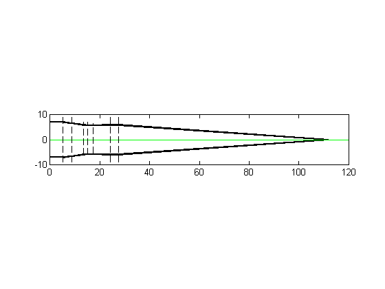
graphical display

z = [0 5 5+cumsum(th)]';
y = [7; py(:,1)];
% make top and bottom a continuous plot
plot([z; flipud(z)],[y; -flipud(y)],'k','LineWidth',2);
axis equal
axis([0 120 -10 10]);

hold on
% optical axis
plot([0 120],[0 0],'g');
% plot surface positions
for k=1:n
    zt = z(k+1);
    plot([zt zt],[-sa(k) sa(k)],'k--');
end
hold off

Published with MATLAB® 7.10