sys1.m

demonstrate sysmatrix and conjugate calculations

Contents

define lens

% define lens (thickness, index, curvature, aperture height)
clear all
close all
th=[0 3.0486 5.4981 1.0162 0.6215 4.6129  3.0486  0 ];
rn=[1  1.713   1      1.689   1      1       1.713  1];
ap=[0  9   9 7.5 7.5 0 9 9 0];
cv=[0  0.0458621 0.0039265 -0.0301655 0.0454845 0 0.0104227 -0.0406946];
lp = find(rn>1);

system matrix

% calculate system matrix
f = sysmatrix(cv,th,rn)

f =

    0.8285   -0.0200
   17.6707    0.7806

% determinant of matrix
det(f)

ans =

     1

% effective focal length (from system matrix)
efl = -1/f(1,2)

efl =

   50.0190

conjugates

Conjugates are calculated as distance from object conjugate to the first lens surface and from the last lens surface to the image conjugate.

% find focal plane (zero magnification)
bfd = conjugates(0,f)

bfd =

      -Inf   41.4387

% find principal planes (unit magnification)
pp = conjugates(1,f)

pp =

  -10.9727   -8.5803

% calculate effective focal length
% (distance from principal plane to focal plane)
efl = bfd - pp

efl =

      -Inf   50.0190

% calculate hiatus (distance between principal planes)
hiatus = sum(th) + sum(pp)

hiatus =

   -1.7070

% planes for 1:1 imaging ( m = -1)
s = conjugates(-1,f)

s =

   89.0652   91.4577

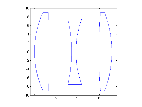
draw lens

drawsys(ap,th,cv,lp);
axis([-1 19 -10 10]);

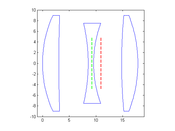
show principal planes

drawsys(ap,th,cv,lp);
hold on;
%
sth = sum(th);
% front principal plane in red, rear principal plane in green
plot(-[pp(1) pp(1)],[-5 5],'r--','LineWidth',2);
plot(sth+[pp(2) pp(2)],[-5 5],'g--','LineWidth',2);
axis([-1 19 -10 10]);
hold off

Published with MATLAB® 7.10