Calibration example

You may find the MATLAB utility files in src.zip useful.

• Open the Calibration GUI

Download the toolbox and unpack to a low-level directory. In my case the path is C:\ece564\bouguet\cam_calib. Edit startup_calib.m. Run this script to add the toolbox to your MATLAB path. Download the images from 2012_0524.zip into an empty folder, move to the folder with the calibration images. Run calib_gui



• Reading the images:

  Click on the Read Images button in the Camera calibration tool window. Enter the basename of the calibration images (2012_0524_) and the image format (jpg).
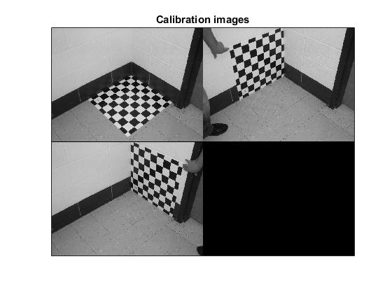
  All the images (three in this case) are then loaded in memory (through the command read images that is automatically executed) in the variables I_1, I_2 , I_3.
  The number of images is stored in the variable n_ima (=3 here).
  

  The matlab figure should look like this:

  

  If the OUT OF MEMORY error message occurred during image reading, that means that your computer does not have enough RAM to hold the entire set of images in local memory. This can easily happen of you are running the toolbox on a 128MB or less laptop for example. In this case, you can directly switch to the memory efficient version of the toolbox by running calib_gui and selecting the memory efficient mode of operation. The remaining steps of calibration (grid corner extraction and calibration) are exactly the same. Note that in memory efficient mode, the thumbnail image is not displayed since the calibration images are not loaded all at once.

• Extract the grid corners:

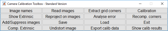
Click on the Extract grid corners button in the Camera calibration tool window.

Extraction of the grid corners on the images
Number(s) of image(s) to process ([] = all images) = >> 

Press "enter" (with an empty argument) to select all the images (otherwise, you would enter a list of image indices like [2 5 8 10 12] to extract corners of a subset of images). Then, select the window size of the corner finder: wintx=winty=16 by entering 16 to the wintx and winty question. This leads to a effective window of size 33x33 pixels.



Window size for corner finder (wintx and winty):
wintx ([] = 16) = >> 
winty ([] = 16) = >> 
Window size = 33x33
Do you want to use the automatic square counting mechanism (0=[]=default)
  or do you always want to enter the number of squares manually (1,other)? >> 

The corner extraction engine includes an automatic mechanism for counting the number of squares in the grid. This tool is specially convenient when working with a large number of images since the user does not have to manually enter the number of squares in both x and y directions of the pattern. On some very rare occasions however, this code may not predict the right number of squares. This would typically happen when calibrating lenses with extreme distortions. At this point in the corner extraction procedure, the program gives the option to the user to disable the automatic square counting code. In that special mode, the user would be prompted for the square count for every image. In this present example, it is perfectly appropriate to keep working in the default mode (i.e. with automatic square counting activated), and therefore, simply press "enter" with an empty argument. (NOTE: it is generally recommended to first use the corner extraction code in this default mode, and then, if need be, re-process the few images with "problems")

Do you want to use the automatic square counting mechanism (0=[]=default)
  or do you always want to enter the number of squares manually (1,other)? >> 

Processing image 1...
Using (wintx,winty)=(16,16) - Window size = 33x33      (Note: To reset the window size, run script clearwin)
Click on the four extreme corners of the rectangular complete pattern (the first clicked corner is the origin)...

The first calibration image is then shown below:



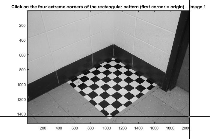
Click on the four extreme corners on the rectangular checkerboard pattern. The clicking locations are shown on the four following figures (WARNING: try to click accurately on the four corners, at most 5 pixels away from the corners. Otherwise some of the corners might be missed by the detector).

Ordering rule for clicking: The first clicked point is selected to be associated to the origin point of the reference frame attached to the grid. The other three points of the rectangular grid can be clicked in any order. This first-click rule is especially important if you need to calibrate externally multiple cameras (i.e. compute the relative positions of several cameras in space). When dealing with multiple cameras, the same grid pattern reference frame needs to be consistently selected for the different camera images (i.e. grid points need to correspond across the different camera views).

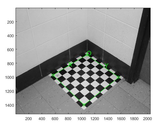
The boundary of the calibration grid is then shown on Figure 2:



number of squares X 7 Y 7

Enter the sizes dX and dY in X and Y of each square in the grid (in this case, dX=dY=3:



Size dX of each square along the X direction ([]=100mm) = >> 3
Size dY of each square along the Y direction ([]=100mm) = 3

Note that you could have just pressed "enter" with an empty argument to select the default values. The program automatically counts the number of squares in both dimensions, and shows the predicted grid corners in absence of distortion:



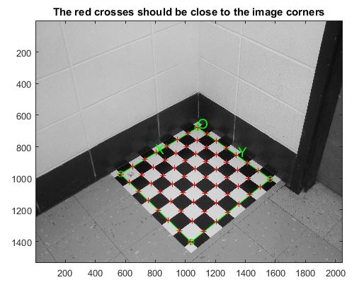
If the guessed grid corners (red crosses on the image) are not close to the actual corners,
it is necessary to enter an initial guess for the radial distortion factor kc (useful for subpixel detection)
Need of an initial guess for distortion? ([]=no, other=yes)

If the predicted corners are close to the real image corners, then this step may be skipped (if there is not much image distortion). This is the case in that present image: the predicted corners are close enough to the real image corners. Therefore, it is not necessary to "help" the software to detect the image corners by entering a guess for radial distortion coefficient. Press "enter", and the corners are automatically extracted using those positions as initial guess.

Corner extraction...

The image corners are then automatically extracted, and displayed as shown below (the blue squares around the corner points show the limits of the corner finder window):



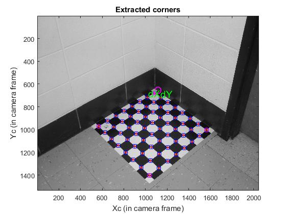
The corners are extracted to an accuracy of about 0.2 pixel.

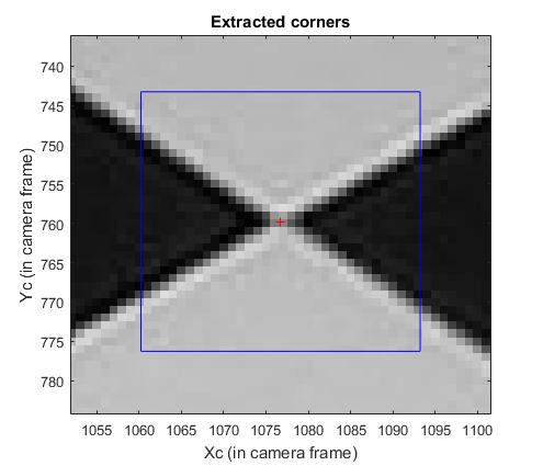
You can zoom in (using MATLAB figure tools) to a portion of the checkerboard, as shown below



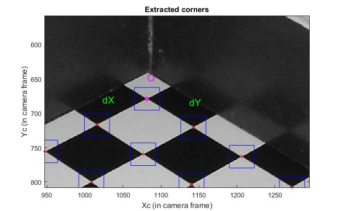
or below (even more detail)



Follow the same procedure for the other images.

• Main Calibration step:

After corner extraction, click on the button Calibration of the Camera calibration tool to run the main camera calibration procedure. Calibration is done in two steps: first initialization, and then nonlinear optimization.
The initialization step computes a closed-form solution for the calibration parameters based not including any lens distortion (program name: init_calib_param.m).The non-linear optimization step minimizes the total reprojection error (in the least squares sense) over all the calibration parameters (9 DOF for intrinsic: focal, principal point, distortion coefficients, and 6*3 DOF extrinsic => 27 parameters). For a complete description of the calibration parameters, click on that link. The optimization is done by iterative gradient descent with an explicit (closed-form) computation of the Jacobian matrix (program name: go_calib_optim.m).



WARNING: The principal point estimation may be unreliable (using less than 5 images for calibration).
Aspect ratio optimized (est_aspect_ratio = 1) -> both components of fc are estimated (DEFAULT).
Principal point optimized (center_optim=1) - (DEFAULT). To reject principal point, set center_optim=0
Skew not optimized (est_alpha=0) - (DEFAULT)
Distortion not fully estimated (defined by the variable est_dist):
     Sixth order distortion not estimated (est_dist(5)=0) - (DEFAULT) .
Initialization of the principal point at the center of the image.
Initialization of the intrinsic parameters using the vanishing points of planar patterns.

Initialization of the intrinsic parameters - Number of images: 3

Calibration parameters after initialization:

Focal Length:          fc = [ 2571.96836   2571.96836 ]
Principal point:       cc = [ 1023.50000   767.50000 ]
Skew:             alpha_c = [ 0.00000 ]   => angle of pixel = 90.00000 degrees
Distortion:            kc = [ 0.00000   0.00000   0.00000   0.00000   0.00000 ]

Main calibration optimization procedure - Number of images: 3
Gradient descent iterations: 1...2...3...4...5...6...7...8...9...10...11...12...13...14...15...16...17...18...19...20...21...done
Estimation of uncertainties...done


Calibration results after optimization (with uncertainties):

Focal Length:          fc = [ 2523.94224   2507.20536 ] ± [ 8.31972   8.98468 ]
Principal point:       cc = [ 960.69629   780.89356 ] ± [ 14.57632   16.16431 ]
Skew:             alpha_c = [ 0.00000 ] ± [ 0.00000  ]   => angle of pixel axes = 90.00000 ± 0.00000 degrees
Distortion:            kc = [ -0.18509   0.48400   -0.00706   -0.00572  0.00000 ] ± [ 0.01685   0.12889   0.00159   0.00136  0.00000 ]
Pixel error:          err = [ 0.15170   0.23660 ]

Note: The numerical errors are approximately three times the standard deviations (for reference).

The Calibration parameters are stored in a number of variables. For a complete description of them, visit this page. Notice that the skew coefficient alpha_c and the 6th order radial distortion coefficient (the last entry of kc) have not been estimated (this is the default mode). Therefore, the angle between the x and y pixel axes is 90 degrees. In most practical situations, this is a very good assumption. However, later on, a way of introducing the skew coefficient alpha_c in the optimization will be presented.

Observe that 21 gradient descent iterations are required in order to reach the minimum. This means 21 evaluations of the reprojection function + Jacobian computation and inversion. The speed of convergence depends on the quality of the initial guess for the parameters computed by the initialization procedure.

• Reproject on Images

Click on Reproject on images in the Camera calibration tool to show the reprojections of the grids onto the original images. These projections are computed based on the current intrinsic and extrinsic parameters. Input an empty string (just press "enter") to the question Number(s) of image(s) to show ([] = all images) to indicate that you want to show all the images:



Number(s) of image(s) to show ([] = all images) = >>

The following figures shows the three images with the detected corners (red crosses) and the reprojected grid corners (circles).



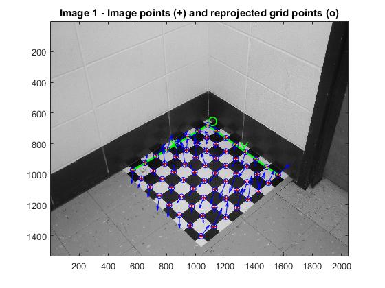
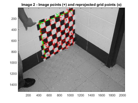
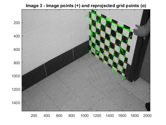
Number(s) of image(s) to show ([] = all images) = >> 
Pixel error:      err = [0.15170   0.23660] (all active images)

• Analyse Error

Click on Analyse Error in the Camera calibration tool to show the reprojection errors in a a scatter diagram.



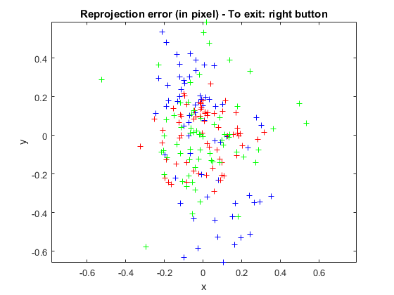
In order to exit the error analysis tool, right-click on anywhere on the figure.

• Show Extrinsics

Click on Show Extrinsic in the Camera calibration tool. The extrinsic parameters (relative positions of the grids with respect to the camera) are then shown in a form of a 3D plot:





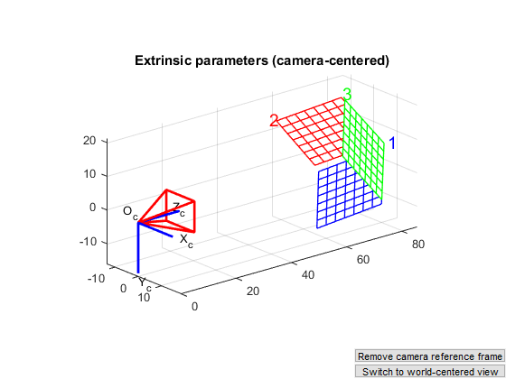
On this figure, the frame (O_c,X_c,Y_c,Z_c) is the camera reference frame. The red pyramid corresponds to the effective field of view of the camera defined by the image plane.

• Save Calibration Results

Click on Save to save the calibration results (intrinsic and extrinsic) in the matlab file Calib_Results.mat .

Publish Results

Publish calib_publish.m to summarize the calibration results.