Download code from bipolar.zip
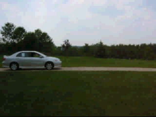
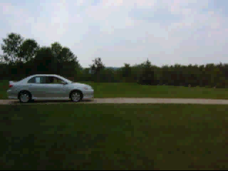
Two images of the same scene are shown below
Careful examination shows that the automobile moves slightly between the two images. Normal images (converted to gray-scale and normalized) vary from zero to one, where zero is black, one is white, and intermediate values are gray.
If these images are subtracted, the resulting values range from a minimum of −1 to a maximum of +1. Values less than zero will be displayed as black.
If diff = g2 - g1, where g1 and g2 are
the grayscale images, we can rescale the difference to the range 0 – 1 by
calculating
g = (diff+1)/2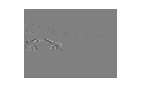
Zero-difference values are medium gray. Negative differences are darker (toward black) and positive differences lighter (toward white).
The MATLAB function bipolar_image.m
does this with g = bipolar_image(diff,0).
Here we code negative values as shades of blue, and positive values as shades of red. Black is the zero difference reference.
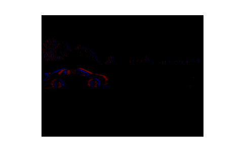
The MATLAB function bipolar_image.m
does this with g = bipolar_image(diff,1).
We again code negative values as shades of blue, and positive values as shades of red. Now, however, white is the zero difference reference.

The MATLAB function bipolar_image.m
does this with g = bipolar_image(diff,2).
We still code negative values as shades of blue, and positive values as shades
of red. Values where abs(diff)<0.3 use the grayscale values of the first
image.
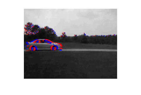
The MATLAB function imdiff.m
does this with g = imdiff(g1,g2).